VLOOKUP (vertical) and HLOOKUP (horizontal) were the only functions available to query a database for specific information. For example, you could query to find and extract all records that contained sales greater $1000 but less than $5000—but only on flat files (only one database matrix).
Pivot Tables were developed so users could create relational databases, which are easier to query, use less memory, and provide more accurate results. If, however, you don’t have or need a relational database, but require more powerful and reliable database functions, try these for a start.
Index, Match, and Index Match
In Excel, the INDEX function returns an item from a specific position (in a list, table, database).The MATCH function returns the position of a value (in a list, table, database). And, the INDEX-MATCH functions used together make extracting data from a table a breeze.
The syntax for the INDEX function is: INDEX(array, row_num, [column_num]). The array is the range of cells that you’re working with. Row_num is, obviously, the row number in the range that contains the data you’re looking for. Column_num is the column number in the range that contains the data you’re looking for. The INDEX formula doesn’t recognize column letters, so you must use numbers (counting from the left).
The syntax for the MATCH function is: MATCH(lookup_value, lookup_array, [match_type]). The lookup_value is the number or text you’re looking for, which can be a value, a logical value, or a cell reference. The lookup_array is the range of cells you’re working with. The match_type determines the MATCH function—that is, an exact match or the nearest match.
A. INDEX function
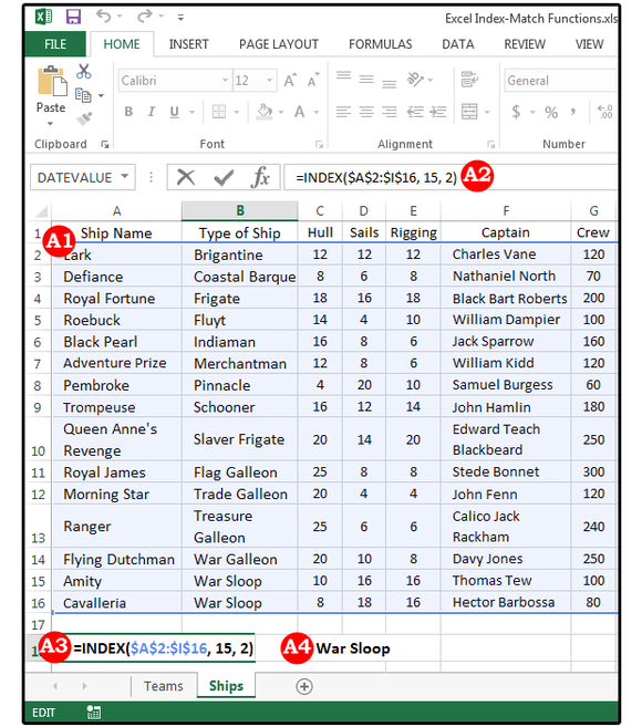
In our example, the famous Commodore James Norrington has a spreadsheet that tracks all the pirate ships in the Caribbean. Norrington’s list is arranged by the ships’ combat formations, which match his nautical charts of the area. When he sees a vessel advancing, he enters the Index formula into his spreadsheet, so he can identify the ship and its capacities. In this first query, Norrington wants to know the type of ship that’s advancing.1. Select a location (cell or range of cells) for your queries (that is, functions and results), then move your cursor to that cell. For example: any cell on row 18.
2. Enter the INDEX function (preceded by the equal sign), plus an opening parenthesis, then highlight (or type) the database/table range like this: =INDEX(A2:I16
Note: If you want an absolute reference (which, in this case, means hard-coding the formula so when/if it’s copied, the range is not altered), press F4 once after each cell reference. You could also highlight the range: Just press F4 once after you select the full range, and the complete absolute reference symbols are added.
3. Next, enter a comma to separate the arguments (that is, the separate formula pieces); then enter the row number and a comma, followed by the column number (yes, it must be a number and not the usual column letter) and the right parenthesis (or just press Enter and let Excel add the ending parenthesis for you). The complete formula looks like this: =INDEX($A$2:$I$16,15,2).
Note: The row numbering starts with the first number in the range, not the first number on the spreadsheet. For example, even though the Cavalleria pirate ship is on Excel row 16, it’s actually row 15 in our formula because our range begins on A2 and goes through I16. If A2 is row 1, then A16 is row 15).
4. Note that the type of ship Norrington was looking for is a War Sloop.
 JD Sartain
 B. INDEX ranges
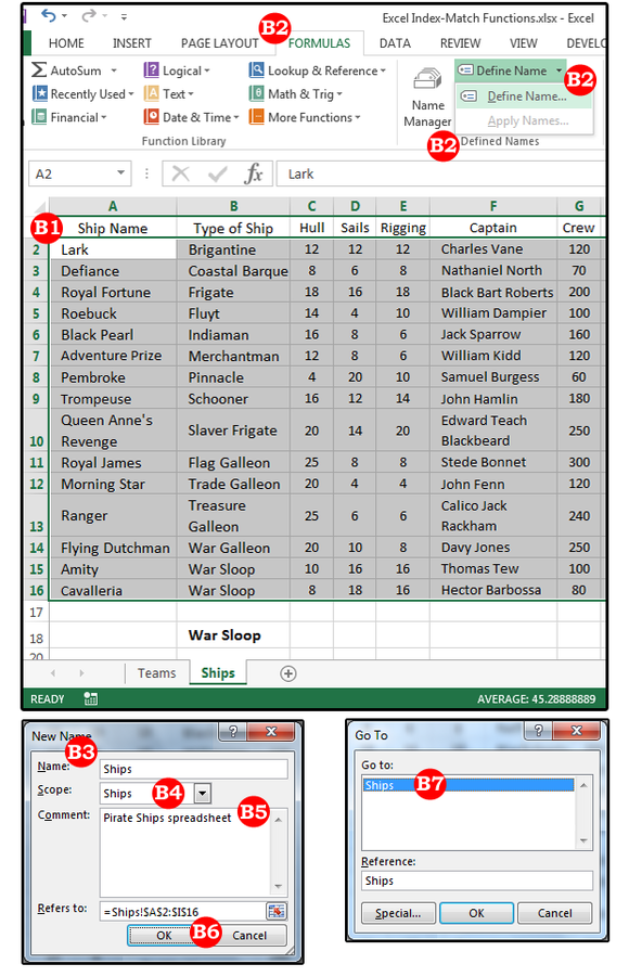
Now, we can do lots more with this database table. You don’t need to redefine the range every time you want to know something. To make it easy, we’ll define the range one time and then name it. Then we can just put the name of the range in our formulas.1. Go to A2 and highlight the range A2 through I16.
2. From the Formulas tab, select Define Name from the Defined Names group.
3. In the popup dialog box, enter a name for your range in the Name field box.
4. Next, enter the Scope (where the range is located), which is either the Workbook or one of the worksheets in the Workbook.
5. Enter a comment, if necessary.
6. And last, verify that the Refers To field displays the correct name and range, then click OK.
7. If you’d like to verify that your range is, indeed, saved in Excel, try this little test: Press Ctrl+G (the GoTo command). Select Ships in the GoTo dialog, then click OK, and Excel re-highlights the range A2:I16.
C. INDEX with SUM & AVERAGE formulas
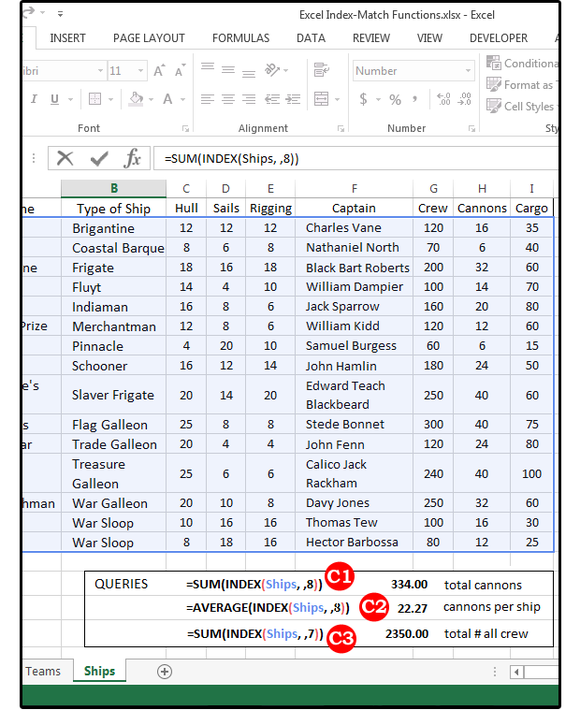
Norrington is assessing the fleet’s battle capabilities. First he wants to know how many cannons the pirates have, the average number of cannons per ship, and the total number of crew manning all those pirate ships. He enters the following formulas:1. =SUM(INDEX(Ships, ,8)) equals 334, the total number of cannons, and
2. =AVERAGE(INDEX(Ships, ,8)) equals 22.27, or approximately 22.27 cannons per ship.
3. =SUM(INDEX(Ships, ,7)) equals 2350, the total number of all crew on all ships.
Why is there a comma, space, comma between Ships and the number 8, and what do these numbers mean? Ships is the Range (followed by a comma), the Row argument is blank (or a space) because Norrington wants all rows, and the 8 represents the 8th column over (which is column H, Cannons).
Some might ask, why not just enter the SUM and/or AVERAGE formulas at the bottom of those columns? In this tiny spreadsheet, yes, it would be just as easy. But if the spreadsheet has 5000 rows and 300 columns, you’ll want to use INDEX
 JD Sartain
 He doesn’t have to visually see his huge database of 5000 records or wait for several seconds while the formulas calculate. He can get all the information he needs from his Query Sheet. Remember, the bigger the spreadsheet, the slower it functions, especially if there are a lot of formulas.
 JD Sartain
 D. INDEX MATCH with MAX
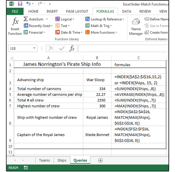
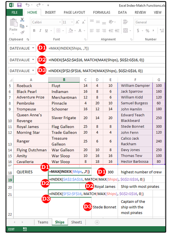
Now, Norrington wants to know how many pirates are on the most populated ship, and which ship is it? He uses the INDEX with MAX formula to get the highest number of pirates, but he also needs to know which ship is carrying them. So he uses the INDEX/MATCH with MAX formula to find out which ship has the most pirates on board.1. =MAX(INDEX(Ships, ,7)) equals 300, the highest number of pirates on one of the ships
2. =INDEX($A$2:$A$16, MATCH(MAX(Ships), $G$2:G$16, 0)) equals the Royal James, the ship with the most pirates aboard
3. =INDEX($F$2:$F$16, MATCH(MAX(Ships), $G$2:G$16, 0)) equals Stede Bonnet, Captain of the Royal James with a pirate crew of 300
 JD Sartain
 Source: http://www.pcworld.com/article/2999860/software/use-index-and-match-for-simple-database-queries-in-excel.html?token=%23tk.PCW_nlt_pcw_powertips_html_2016-03-17&idg_eid=8458d72e614c68751de48f5c175520f4&utm_source=Sailthru&utm_medium=email&utm_campaign=PCWorld%20Power%20Tips%202016-03-17&utm_term=pcw_powertips_html#tk.PCW_nlt_pcw_powertips_html_2016-03-17