jfn Excel & accounting tips: May 2014

By Mary Richardson March 29, 2005, 6:17 PM PST

Tired of opening Excel from your desktop shortcut and seeing an empty workbook? Then follow these step-by-step instructions to create an application that will not display an empty workbook.

Help users increase productivity by automatically signing up for TechRepublic's free Microsoft Office Suite newsletter, featuring Word, Excel, and Access tips, delivered each Wednesday.

If you normally launch Excel 2002 by clicking a shortcut on your desktop, you may not want to see an empty workbook. To prevent Excel from displaying an empty workbook when it is started, follow these steps:

In Windows Explorer, go to \Program Files\Microsoft Office\Office10\Shortcut bar\Office and delete the existing shortcut for Excel. (In Excel 2003, go to \Program Files\Microsoft Office\Office11\Shortcut bar\Office.)
In Windows Explorer, go to \Program Files\Microsoft Office\Office10. Then, right-click the EXCEL.exe icon and select Create Shortcut. (In Excel 2003, go to \Program Files\Microsoft Office\Office11. Then, right-click the EXCEL.exe icon and select Create Shortcut.)
Right-click the shortcut icon and select Properties.
In the Shortcut tab, add a space, followed by the /e switch to the path in the Target box. For example, in Excel 2002, the entry in the Target box would be: "C:\Program Files\Microsoft Office\Office10\EXCEL.exe" /e
Click OK.

When you double-click the Excel shortcut icon, the application will open without displaying a blank workbook.

Source: http://www.techrepublic.com/article/open-excel-without-a-blank-workbook/

Julie Sartain

May 30, 2014 3:30 AM
print

One of Excel’s greatest tricks is the dimensional or 3D reference. This feature, which allows you to create formulas that refer to the same cell or range on multiple worksheets, simplifies the creation of complex documents like monthly inventories or sales reports. In Excel 2013, Microsoft has beefed it up with enhanced options and formulas.
To illustrate the power and flexibility of 3D worksheets, we’ll create a Year-to-Date project that calculates the utility bills for a small business for each month, with the year-to-date totals on the first sheet. This workbook (which contains of all the worksheets in this project) calculates the columns, rows, and multiple spreadsheets three-dimensionally.
Because retyping the same data is counterproductive, we’ll create the month of January first, add the formulas for the columns and rows, and then copy this sheet 12 times (one for each month, plus the year-to-date sheet).
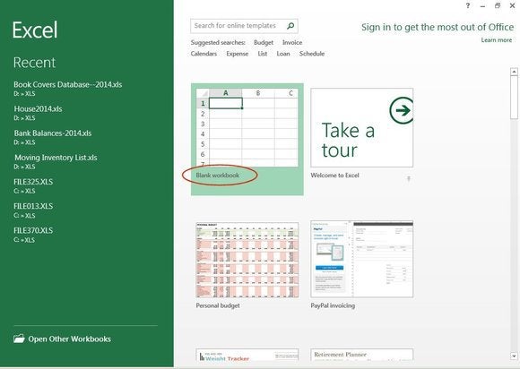
Start by selecting Blank workbook from the Home menu page.

f1 excelhomemenu blank workbook — In Excel 2013 Home Menu, select *Blank workbook*.

Sheet title and custom date

In cell A1, type January 2014. Excel changes the format to Jan-14. Right-click the mouse in that cell and choose Format Cells from the dropdown list. Choose Date from the format options, and you’ll notice that there is not a format listed for the month spelled out with a four-digit year. Choose Custom and in the Type field box above the list enter mmmm yyyy, then click OK. Now your title says 'January 2014.'
This small business has four designers who rent space. The rent is divided equally, but the utilities and other fees are calculated by percentages of use, therefore each designer pays a different price. Be sure to use the actual percent sign when you enter these numbers.

Enter data and format cells

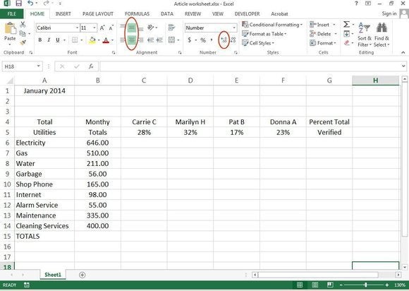
In cells A4 through G4 enter this data: Total, Monthly, Carrie C, Marilyn H, Pat B, Donna A, and Percent Total. In cells A5 through G5 enter this data: Utilities, Totals, 28%, 32%, 17%, 23%, and Verified. Select cells A4 through G5 and click Center from the Ribbon bar on the Home menu tab. Note: You can center both horizontally and vertically.
In cells A6 through A15, enter this information: Electricity, Gas, Water, Garbage, Shop Phone, Internet, Alarm Service, Maintenance, Cleaning Services, TOTALS. Adjust column widths to fit the data entered. In B6 through B14, enter these numbers: 646, 510, 211, 56, 165, 98, 55, 335, and 400. Select cells B6 through G15, then click Center, and then click Increase Decimal (two times) to format for two decimal places (both on the Home menu tab).

f2 enter dataformat cells — Enter worksheet data and format the cells.

Add formulas

This part is really easy and, by copying all the formulas, really fast. In cell C6 enter this formula:
=sum(B6*C5) and click Enter. With your cursor on C6, press F2 to edit the formula. Position your cursor before the 'B' in 'B6' (between the left parenthesis and the B), then press F4 three times—until you see a dollar sign appear in front of the letter 'B.' Still in edit mode, move the cursor to the left of the letter C in C5 and press F4 twice (until you see a dollar sign appear in front of the number 5), then press Enter. Your formula in C6 should look like this: =sum($B6*C$5). This little trick locks the pieces of the formula (that is, column B and row 5) that you don’t want to change (called absolute reference) and therefore prevents lots of editing.

Copy formulas

Reposition your cursor to C6. Click Copy from the Ribbon bar (or press Ctrl+C). Move your cursor to C7, select cells C7 through C14, then press Enter. With C7 through C14 still selected, click Copy again, move your cursor to D7, select D7 through F14, then press Enter. All the cells will calculate.
Now, to verify that all the calculations are correct (in case there’s a typo somewhere), position the cursor in G6 and enter this formula: =sum(C6:F6) and press Enter (you can also highlight these ranges and let Excel fill in the cell locations). With your cursor on G6, click Copy, select cells G7 through G14, and press Enter. If the numbers in column G match the numbers in column B exactly, then your formulas are all correct.
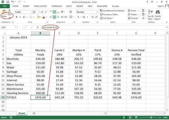
Next, position your cursor on cell B15 and enter this formula: =sum(B6:B14) and press Enter. With your cursor on B15, click Copy, select cells C15 through G15, and press Enter.

Copy and rename spreadsheets

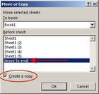
f4 copy spreadsheets — Copy Spreadsheet 12 Times.

Copy this spreadsheet 12 times for a full year's worth of data. Place your cursor on the Sheet1 tab at the bottom of your Excel window. Right-click the mouse and select Move or Copy from the drop list. Check the box that says Create a Copy, select (move to end), then click OK.
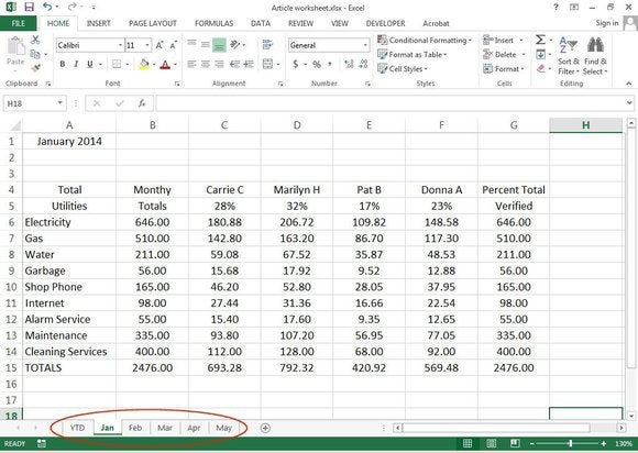
Double-click the tab that says Sheet1 and rename it YTD. Double-click the remaining sheet tabs Sheet1 (2) through Sheet1 (12) and rename the worksheet tabs Jan, Feb, Mar, etc., through Dec. Next, change the titles of each sheet to match the tabs (type over 'January 2014' with correct titles). Note: Keep spreadsheet tab titles as short as possible for easier dimensional calculating.

f5 rename spreadsheets — Rename spreadsheets and spreadsheet tabs.

Access spreadsheets Feb through Dec and enter some random numbers in the Monthly Totals column—cells B6 through B14 (not B15, because it’s a formula). For this example, the dimensional totals only calculate Jan through May.

Add 3D worksheet formulas

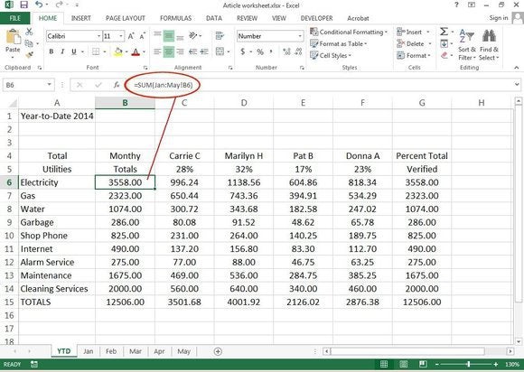
On the YTD spreadsheet, position your cursor on B6 and enter this formula: =sum(Jan:Dec!B6). Copy this formula from B6 down to B7 through B14 (not B15, because this formula totals this column).

f6 addcopy 3d spreadsheet formulas — Add formulas to total spreadsheets dimensionally from Jan through Dec.

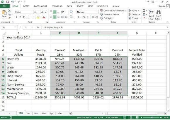
Next, select cells B6 through B14, select Copy, then highlight C6 through F14 and press Enter. The YTD spreadsheet now has the totals from the entire year. Every time you make a change in column B (Monthly Totals) on spreadsheets Jan through Dec—that is, every time you make an adjustment to the individual utility fees—the entire spreadsheet recalculates to reflect those new numbers.

f7 addcopy 3d spreadsheet formulas2 — Copy dimensional formulas from column B to remaining columns in YTD spreadsheet.

In 2015, delete the numbers in column B from B6 thru B14 on all spreadsheets from Jan through Dec, then enter the correct utility fees each month as the bills arrive. Watch the YTD spreadsheet totals change as it adds each month's totals. Once these spreadsheets are created with the formulas, you’ll never have to repeat this process.

Future edits are easy

If you have to add or remove a utility from a 3D worksheet, be sure to stay inside the calculated area. For example, if the alarm service is discontinued in June of 2015, don’t change anything. Just enter zeros in that cell for July through Dec. Then, in January of 2016, place your cursor on that row (on each spreadsheet, Jan through Dec, including the YTD spreadsheet) and select Delete Sheet Row (from the Home menu tab).
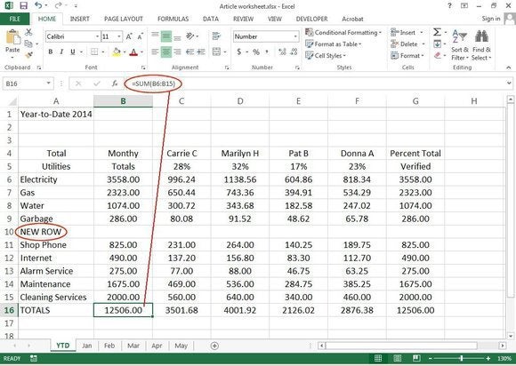
To add a new utility, place your cursor anywhere between cells B6 and B14 and select Insert Sheet Row. Then copy the formulas for that row from the row above it. Inserting new rows inside the matrix ensures that the new row’s numbers and formulas are included in the project-wide formulas. If rows are inserted outside the matrix, the numbers and formulas on this row will not be included in any of your calculations unless you adjust all your formulas to include this new range.
Note that when you insert a new row between B6 and B14, the TOTALS row moves down to B16, and the formula in that cell (which totals column B) changes from =sum(B6:B14) to =sum(B6:B15). Stay inside the original matrix range, and everything will calculate accurately throughout the entire project.

f8 adddelete rows — Stay inside the original spreadsheet matrix when adding or deleting rows.

Source: http://www.pcworld.com/article/2241304/how-to-create-3d-worksheets-in-excel-2013.html#tk.rss_all

jfn Excel & accounting tips

Friday, May 30, 2014

Open Excel 2013 without a blank workbook

Thursday, May 29, 2014

How to create 3D Worksheets in Excel 2013