This is where the number-crunching fun
starts. Learn the ins and outs of the logical formulas that represent
the heart of Excel.
Excel functions, or formulas, lie at the heart of the application’s deep
well of capabilities. Today we’ll tackle IF statements, a string of
commands that determine whether a condition is met or not. Just like a
yes-no question, if the specified condition is true, Excel returns one
user-determined value and, if false, it returns another.
The IF statement is also known as a logical formula: IF, then, else. If something is true, then do this, else/otherwise do that. For example, if it’s raining, then close the windows, else/otherwise leave the windows open.
The syntax (or sentence structure; that is, the way the commands are
organized in the formula) of an Excel IF statement is: =IF(logic_test,
value_if true, value_if_false). IF statements are used in all
programming languages and, although the syntax may vary slightly, the
function provides the same results.
Remember: Learning Excel functions/formulas and how they work are the
first steps toward using Visual Basic, Microsoft’s event-driven
programming language. Here are five easy IF statements to get you
started.
Past-due notices
Use an IF statement to flag past-due accounts so you can send notices to those customers.
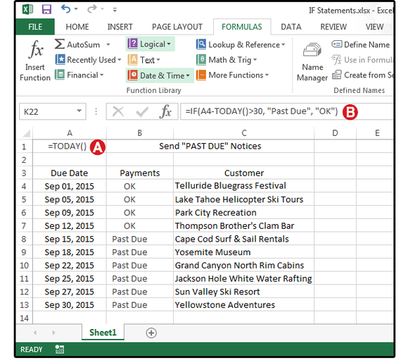
In this spreadsheet, the customer’s payment due date is listed in column
A, the payment status is shown in column B, and the customer’s company
name is in column C. The company accountant enters the date that each
payment arrives, which generates this Excel spreadsheet. The bookkeeper
enters a formula in column B that calculates which customers are more
than 30 days past due, then sends late notices accordingly.
A. Enter the formula: =TODAY() in cell A1, which displays as the current date.
B. Enter the formula: =IF(A4-TODAY()>30, “Past Due”, “OK”) in cell B4.
In English, this formula means: If the date in cell A4 minus today’s date is greater than 30 days, then enter the words ‘Past Due’ in cell B4, else/otherwise enter the word ‘OK.’ Copy this formula from B4 to B5 through B13.
Pass/Fail lifeguard test
Use an IF statement to convert numeric scores to a pass-fail status.
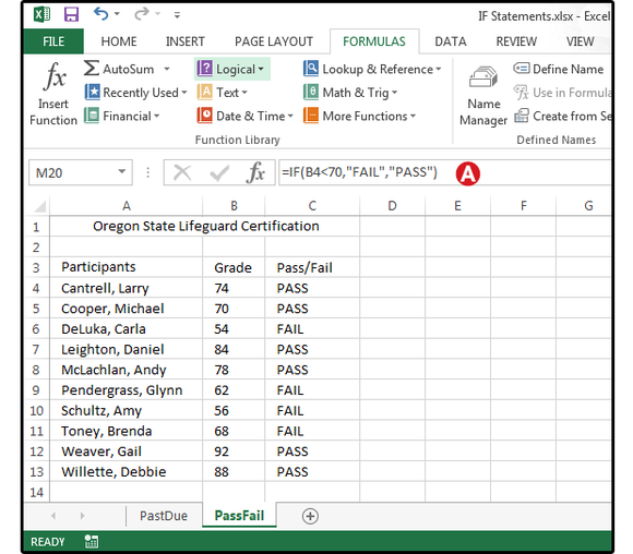
The Oregon Lifeguard Certification is a Pass/Fail test that requires
participants to meet a minimum number of qualifications to pass. Scores
of less than 70 percent fail, and those scores greater than that, pass.
Column A lists the participants’ names; column B shows their scores; and
column C displays whether they passed or failed the course. The
information in column C is attained by using an IF statement.
Once the formulas are entered, you can continue to reuse this
spreadsheet forever. Just change the names at the beginning of each
quarter, enter the new grades at the end of each quarter, and Excel
calculates the results.
A. Enter this formula in cell C4: =IF(B4<70,”FAIL”,”PASS”). This means if the score in B4 is less than 70, then enter the word FAIL in cell B4, else/otherwise enter the word PASS. Copy this formula from C4 to C5 through C13.
Sales & bonus commissions
Use an IF statement to calculate sales bonus commissions.
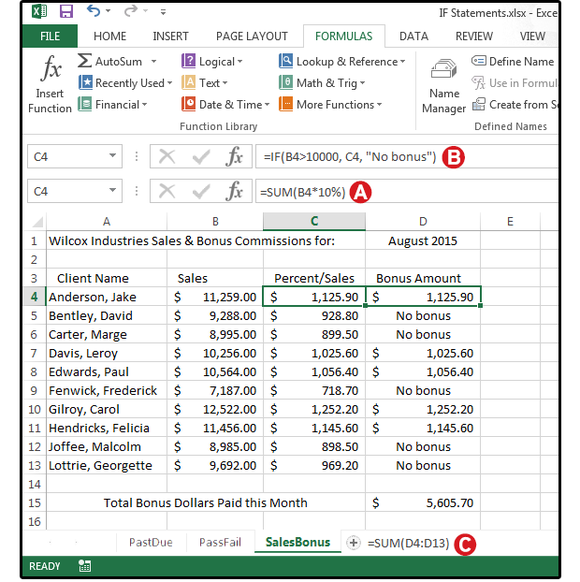
Wilcox Industries pays its sales staff a 10-percent commission for all
sales greater than $10,000. Sales below this amount do not receive a
bonus. The names of the sales staff are listed in column A. Enter each
person’s total monthly sales in column B. Column C multiples the total
sales by 10 percent, and column D displays the commission amount or the
words 'No Bonus.' Now you can add the eligible commissions in column D
and find out how much money was paid out in bonuses for the month of
August.
A. Enter this formula in cell C4: =SUM(B4*10%), then copy from C4 to C5 through C13. This formula calculates 10 percent of each person’s sales.
B. Enter this formula in cell D4: =IF(B4>10000, C4, “No bonus”),
then copy from D4 to D5 through D13. This formula copies the percentage
from column C for sales greater than $10,000 or the words 'No Bonus'
for sales less than $10,000 into column D.
C. Enter this formula in cell D15: =SUM(D4:D13). This formula sums the total bonus dollars for the current month.
Convert scores to grades with nested IF statements
Use a nested IF statement to calculate different commissions based on different percentages.
This example uses a “nested” IF statement to convert the numerical Math
scores to letter grades. The syntax for a nested IF statement is this:
IF data is true, then do this; IF data is true, then do this; IF data is
true, then do this; IF data is true, then do this; else/otherwise do
that. You can nest up to seven IF functions.
The student’s names are listed in column A; numerical scores in Column
B; and the letter grades in column C, which are calculated by a nested
IF statement.
A. Enter this formula in cell C4: =IF(B4>89,”A”,IF(B4>79,”B”,IF(B4>69,”C”,IF(B4>59,”D”,”F”)))), then copy from C4 to C5 through C13.
Note: Every open, left parenthesis in a formula must
have a matching closed, right parenthesis. If your formula returns an
error, count your parentheses.
Determine sliding scale sales commissions with nested IF statements
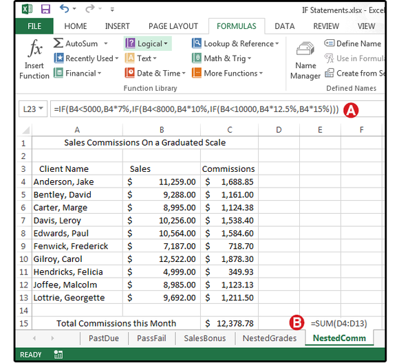
This last example uses another nested IF statement to calculate multiple
commission percentages based on a sliding scale, then totals the
commissions for the month. The syntax for a nested IF statement is this:
IF data is true, then do this; IF data is true, then do this; IF data
is true, then do this; else/otherwise do that. The names of the sales
staff are listed in column A; each person’s total monthly sales are in
column B; and the commissions are in column C, which are calculated by a
nested IF statement, then totaled at the bottom of that column (in cell
C15).
A. Enter this formula in cell C4: =IF(B4<5000,B4*7%,IF(B4<8000,B4*10%,IF(B4<10000,B4*12.5%,B4*15%))), then copy from C4 to C5 through C13.
B. Enter this formula in cell C15: =SUM(C4:C13). This formula sums the total commission dollars for the current month.
Use a nested IF statement to calculate different commissions based on different percentages.
If you have a lot of blank rows in your Excel spreadsheet, you can
delete them by right-clicking each once separately and selecting
“Delete,” a very time-consuming task. However, there’s a quicker and
easier way of deleting both blank rows and blank columns.
First, we’ll show you how to delete blank rows. Deleting blank
columns is a similar process that we’ll show you later in this article.
Highlight the area of your spreadsheet in which you want to delete
the blank rows. Be sure to include the row just above the first blank
row and the row just below the last blank row.
Click “Find & Select” in the “Editing” section of the “Home” tab and select “Go To Special…” on the drop-down menu.
On the “Go To Special” dialog box, select “Blanks” and click “OK.”
All the cells in the selection that are not blank are de-selected, leaving only the blank cells selected.
In the “Cells” section of the “Home” tab, click “Delete” and then select “Delete Sheet Rows” from the drop-down menu.
All the blank rows are removed and the remaining rows are now contiguous.
You can also delete blank columns using this feature. To do so,
select the area containing the blank columns to be deleted. Be sure to
include the column to the left of the leftmost column to be deleted and
the column to the right of the rightmost column to be deleted in your
selection.
Again, click “Find & Select” in the “Editing” section of the “Home” tab and select “Go To Special…” from the drop-down menu.
Select “Blanks” again on the “Go To Special” dialog box and click “OK.”
Again, all the cells in the selection that are not blank are
de-selected, leaving only the blank cells selected. This time, since
there are no blank rows selected, only blank columns are selected.
Click “Delete” in the “Cells” section of the “Home” tab and then select “Delete Sheet Columns” from the drop-down menu.
The blank columns are deleted and the remaining columns are contiguous, just as the rows are.
This method for deleting blank rows and columns is quicker,
especially if you have a large workbook containing large and multiple
worksheets.