Kumar Malyala asked if there’s a way in Excel to count the number of business days between two dates.
It’s easy to find the number of days between two dates in Excel. You
just subtract the earlier date from the later one. If you put July 19 in A1, May 5 in A2, and enter =a1-a2 in A3, you’ll get 75—the number of days between May 5 and July 19.
However, if you don’t want Saturdays and Sundays in your total, you’ll
have to work a bit harder. And if you need to take holidays into
consideration, it gets trickier still.
But not too tricky.
[Have a tech question? Ask PCWorld Contributing Editor Lincoln Spector. Send your query to answer@pcworld.com.]
With or without holidays, you’ll need to use the networkdays function. And no, it has nothing to do with connectivity. The name means net workdays, not network days.
I tested this in Excel 2010 and 2016.
To find the number of weekdays between two dates, simply use the formula =networkdays(Start_date,End_date), with Start_date addressing the cell containing the earlier of the two dates, and End_date addressing the later date. For instance, if you have April 16 in A1 and September 19 in A2, =networkdays(a1,a2) will give you the answer 111.
Keep in mind that networkdays counts the Start_date in its result. If
your Start_date is a Monday, and the End_date is the same week’s Friday,
networkdays will return the number 5, not 4.
To subtract your office’s holidays from the networkdays results, create a
list of company holidays somewhere on the spreadsheet (it can be on a
different tab). The actual dates of the holidays should be listed in a
column.
You’ll need to create what Excel calls a named range of those holiday dates. Select the dates, then go to the Formula ribbon and pick Define Name (Excel 2010) or Defined Names > Define Name (Excel 2016). (For more on named ranges, read JD Sartain's detailed how-to.)
In the resulting dialog box, give the range the name holidays.
Then add the argument holidays to the end of the networkdays formula. In other words, instead of =networkdays(a1,a2), enter =networkdays(a1,a2,holidays).
The weekdays where your office is closed will no longer be counted in the formula.by Lincoln Spector Contributing Editor
When you want to track down a particular record right now,
creating a query for the job is overkill. Fortunately, Access 2016 has a
very simple way to find one specific piece of data in your project’s
tables and forms: the Find command.
Find is found — big surprise here — in the Find section of the Home
tab, accompanied by a binoculars icon. You can also get to Find by
pressing Ctrl+F to open the Find dialog box.
Although the Find command is pretty easy to use, knowing a
few tricks makes it even more powerful, and if you’re a Word or Excel
user, you’ll find the tricks helpful in those applications, too —
because the Find command is an Office-wide feature.
Finding anything fast
Using the Find command is a very straightforward task. Here’s how it works:
Open the table or form you want to search.
Note that the Find command works in Datasheet view
and with Access forms and becomes available as soon as a table or form
is opened.
Click in the field that you want to search.
The Find command searches the current field in all
the records of the table, so be sure to click the correct field before
starting the Find process. Access doesn’t care which record you click;
as long as you’re on a record in the correct field, Access knows exactly
which field you want to Find in.
Start the Find command.
You can either click the Find button in the Find section of the Home tab or press Ctrl+F.
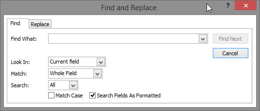
The Find and Replace dialog box opens, ready to serve you.
Type the text you’re looking for in the Find What box.
Take a moment to check your spelling before
starting the search. Access is pretty smart, but it isn’t bright enough
to figure out that you actually meant plumber when you typed plumer.
The Find and Replace dialog box.
Click Find Next to run your search.
If the data you seek is in the active field, the Find command immediately tracks down the record you want.
The cell containing the data you seek is highlighted.
What if the first record that Access finds isn’t
the one you’re looking for? Suppose you want the second, third, or the
fourteenth John Smith in the table? No problem; that’s why the
Find and Replace dialog box has a Find Next button. Keep clicking Find
Next until Access either works its way down to the record you want or
tells you that it’s giving up the search.
If Find doesn’t locate anything, it laments its failure in a small dialog box, accompanied by this sad statement:
Microsoft Access finished searching the records. The search item was not found.
If Find didn’t find what you were looking for, you have a couple of options:
You can give up by clicking OK in the small dialog box to make it go away.
You can check the search and try again
(you’ll still have to click OK to get rid of the prompt dialog box).
Here are things to check for after you’re back in the Find and Replace
dialog box:
Make sure that you clicked in the correct field and spelled everything correctly in the Find What box.
You can also check the special Find options to see whether one of them is messing up your search.
If you ended up changing the spelling or options, click Find Next again.
Shifting Find into high gear
Sometimes just typing the data you need in the Find What box doesn’t produce the results you need:
You find too many records (and end up clicking the Find Next button endlessly to get to the one record you want).
The records that match aren’t the ones you want.
The best way to reduce the number of wrong matches is to add more
details to your search, which will reduce the number of matches and
maybe give you just that one record you need to find.
Access offers several tools for fine-tuning a Find. To use them, open the Find and Replace dialog box by either
Clicking the Find button on the Home tab
or
Pressing Ctrl+F
If your Find command isn’t working the way you think it should, check
the following options. Odds are that at least one of these options is
set to exclude what you’re looking for.
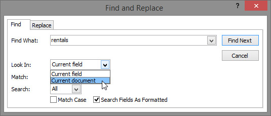
Look In
By default, Access looks for matches only in the current field
— whichever field you clicked in before starting the Find command. To
tell Access to search the entire table instead, choose Current Document
from the Look In drop-down list.
To search the entire table, change Look In.
Match
Your options are as follows:
Any Part of Field: Allows a match anywhere in a field (finding Richard, Ulrich, and Lifestyles of the Rich and Famous). This is the default.
Whole Field: This requires that the search terms (what you type in the Find What box) be the entirety of the field value. So Rich won’t find Ulrich, Richlieu, Richard, or Richmond. It finds only Rich.
Start of Field: Recognizes only those matches that start from the beginning of the field. So Rich finds Richmond, but not Ulrich.
This option allows you to put in just part of a
name, too, especially if you know only the beginning of a name or the
start of an address.
To change the Match setting, click the down arrow next to the Match
field and then make your choice from the drop-down menu that appears.
Using the Match option.
Search
If you’re finding too many matches, try limiting your search to one
particular portion of the table with the help of the Search option.
Search tells the Find command to look either
At all the records in the table (the default setting)
or
Up or down from the current record
Clicking a record halfway through the table and then telling Access
to search Down from there confines your search to the bottom part of the
table.
Fine-tune your Search settings by clicking the down arrow next to the
Search box and choosing the appropriate offering from the drop-down
menu.
Match Case
Checking the Match Case check box makes sure that the term you search for is exactly the same as the value stored in the database, including the same uppercase and lowercase characters.
This works really well if you’re searching for a name, rather than just a word, so that rich custard topping is not found when you search for (capital R) Rich in the entire table.
Search Fields as Formatted
This option instructs Access to look at the formatted version of the
field rather than the actual data you typed. By “formatted” this means
with formatting applied to the content – numbers formatted as
percentages, dates set as short dates vs medium dates, and so on.
Limiting the search in this way is handy when you’re searching for
dates, stock-keeping unit IDs, or any other field with quite a bit of
specialized formatting.
Turn on Search Fields as Formatted by clicking the check box next to it.
This setting doesn’t work with Match Case, so if Match
Case is checked, Search Fields as Formatted appears dimmed. In that
case, uncheck Match Case to bring back the Search Fields as Formatted
check box.
Most of the time, this option doesn’t make much difference. In fact,
the only time you probably care about this particular Find option is
when (or if) you search many highly formatted fields.
My March 2 column on continuous accounting,
“Stopping the Madcap Sprint to Close the Books,” apparently struck a
chord, encouraging many readers to write thoughtful responses. Most
wanted to know how continuous accounting “actually works.” This piece is my reply to these inquiries.
First a quick recap of my earlier column: Continuous accounting is a
measured and balanced alternative to compressing a month’s (or more)
worth of accounting tasks to close the books into a few days at the end
of the month, quarter, or year. Rather, the work to perform such closing
tasks is conducted incrementally by accountants during the month, quarter, and year.
The benefits include a reduction in the pile-up of accounting work
and the stress this causes; lower risk of financial irregularities; and
an earlier opportunity for financial planning & analysis to deliver
the business forecast. CFO readers intrigued by these benefits wanted to know, as one wrote, “How does this actually work?”
To answer the question, let’s start with today’s inefficient workload
procedures. As part of their bookkeeping, accountants in midsize and
larger companies manually sift through thousands of spreadsheets
generated by different systems. Without an automated system, it’s an
uphill climb to methodically tick and tie the ledgers to confirm that
every item is accounted for and properly connected to related items.
This confirmation process is therefore pushed off to the end of the
month, quarter, or year.
Another inefficiency derives from batch processing. When digital
documents replaced paper-based accounting records, technological
limitations caused the accounting work to be stored up during working
hours and executed when computer systems were offline. As the volume of
data expanded, the process took more time to run. Ultimately, the system
was not ready to use when accountants required its use. Again, the
solution was to push off the work.
What’s wrong here? Top-notch accounting talent
is underutilized during non-peak periods and overworked during the peak
period. To alleviate some of the workload, finance and accounting hires
temp workers that eat up the budget.
These many inadequacies and the pains they inflicted — from
burned-out accountants and pointless costs to an increased risk of
errors, out-of-date results, and zero time for analysis — raise the
obvious question: “What if we could account for the business at close at
the speed of transactions?”
Well, the answer is, you can.
And Here’s How
The first thing to do is to rethink the internal paradigm of accounting, adjusting the mindset to consider the F&A
process as one of continuous improvement. The goal is to optimize the
accounting process one task at a time, then rinse and repeat. By
building automation and accuracy into the accounting process,
accountants are eliminating the time wasted performing redundant
exercises and fixing errors. In this voyage, automated technology is a
tool to achieve the ends; it is not the beginning of the journey.
Great things are possible once a philosophy of continuous accounting
is in place. Instead of bringing up all the data in one batch process as
before, the batch is split up into a series of smaller tasks. Tasks are
scheduled as early in the accounting process as possible and embedded
within the everyday workflow of the accountants. By breaking the tasks
into smaller pieces, the completion of these elements becomes routine, a
process that takes its cue from agile software development. Tasks are
automated where possible and standardized elsewhere.
The last step is to monitor the effectiveness of these process efficiency improvements through predictive analytics,
measuring the time it takes to close the books, the total costs per
full-time F&A employee, and the average number of days for an
accountant to complete a selected assignment.
Continuous Accounting in Action
Sounds all well and good, but readers have asked for “actual
examples.” Let’s apply the above steps to a particular F&A task —
account reconciliations.
The current state of many finance organizations is to perform the
reconciliations at the end of the month, reducing the opportunity to
conduct proactive analysis before then. The alternative is to split the
batch process into smaller tasks, such as the daily reconciliation of key
accounts. To perform this task earlier, scheduled end-of-month
reconciliations are shifted to event-based reconciliations, i.e., as
they occur. Automation is used to automatically reconcile the key
accounts and match these transactions. Accountants are now in the
position to investigate anomalies associated with these reconciliations
throughout the month, minimizing the period-end rush.
Let’s apply continuous accounting to another routine F&A task —
intercompany accounting, the process of balancing the accounts between
two different company branches to bring the balances to zero in the
general ledger. The current state in most F&A organizations is to
wait until the books are closed and entries are booked by these
different entities before performing the task. Since the time it takes
to record the transactions varies by entity, there’s no time to react to
possible discrepancies, culminating in a rushed review at the
period-end.
By dividing the batch process into smaller tasks, intercompany
transactions can be recorded and approved on each entity’s books in
real-time throughout the period. The task no longer waits until the end
of the month, quarter, or year, as it is embedded along with the proper
controls into daily workflows for automatic approval. By automating this
process, accountants are freed to focus on value-added services to the
CFO.
As the reader can see, continuous accounting is a philosophical
approach, not simply a technological one. Only by first analyzing the
current state of F&A can a vastly more efficient future state be
designed, followed by its development and continuous improvement. Therese Tucker is CEO of financial automation software provider BlackLine.
When
you need to do a speedy analysis of your data in Excel 2016, consider
using the Quick Analysis feature. Here are some points to keep in mind
about Quick Analysis:
When you select a range of
cells, a small icon appears in the lower right corner of the selected
area. This is the Quick Analysis icon, and clicking it opens a panel
containing shortcuts to several types of common activities related to
data analysis.
Click on of the five headings
to see the shortcuts available in that category. Then hover over one of
the icons in that category to see the result previewed on your
worksheet:
Formatting: These
shortcuts point to conditional formatting options. For example, you
could set up a range to make values under or over a certain amount
appear in a different color or with a special icon adjacent.
Open the Quick Analysis panel by clicking its icon. Then choose a category heading and click an icon for a command.
Charts: These shortcuts generate common types of charts based on the selected data.
Quick Analysis offers shortcuts for creating several common chart types.
Totals: These shortcuts add the specified calculation to adjacent cells in the worksheet. For example, Sum adds a total row or column.
Notice that there are separate icons here for rows vs. columns.
Notice also that in this category there are
more icons than can be displayed at once, so there are right and left
arrows you can click to scroll through them.
You can use Quick Analysis to add summary rows or columns.
Tables: You can convert
the range to a table for greater ease of analysis. You can also
generate several different types of PivotTables via the shortcuts here. A
PivotTable is a special view of the data that summarizes it by adding various types of calculations to it.
The PivotTable icons aren’t well-differentiated,
but you can point to one of the PivotTable icons to see a sample of how
it will summarize the data in the selected range. If you choose one of
the PivotTable views, it opens in its own separate sheet.
You can convert the range to a table or apply one of several PivotTable specifications.
Sparklines:Sparklines
are mini-charts placed in single cells. They can summarize the trend of
the data in adjacent cells. They are most relevant when the data you
want to trend appears from left to right in adjacent columns.
Choose Sparklines to add mini-charts that show overall trends.
No one denies that Excel is an incredibly powerful piece of software. Yet, learning how to use its more advanced features is far from easy. With that in mind, we’ve tracked down ten top Excel gurus who can help you master the advanced functions of Excel more easily.
But if you want to take your knowledge even further, you’ll need reliable Excel specialists, who are willing to share their growing, in-depth knowledge of this program with you.
The following ten Excel gurus fit this description perfectly. Each guru regularly publishes step-by-step tutorials that walk you through these more advanced Excel features that you could otherwise be wrestling with for weeks.
Purna Duggirala (aka, “Chandoo”) is a minor celebrity in Excel circles. Since 2004, Chandoo has been regularly sharing everything he learns while working with Excel. His site, which aims to “make you awesome in Excel” now receives over 1.5m visitorsper month, and is Chandoo’s full-time project.
Much of the content on Mynda Treacy’s site is available free of charge. It is made up of in-depth Excel tutorials accompanied by screenshots and videos to really drill home the lessons. These tutorials include more basic lessons, such asselecting multiple items from a data validation list, to advanced tutorials onPower Query reformats.
On the site, you’ll also find a range of top quality webinars run by other Excel professionals that you can stream for no cost.
Having been working with Excel for two decades, Bill Jelen (aka “Mr Excel”) is a true oracle of this software. But if that’s not enough, the huge Excel forum on Jelen’s site houses an army of Excel experts to answer any of your questions.
ExcelIsFun is the huge Excel YouTube channel run by Mike Girvin. With well over 2,000 Excel video tutorials, this is a channel that anyone who regularly works with Excel should subscribe to. Most of the videos are 7-15 minutes long, and are very easy to follow (provided you have a basic grasp of Excel already).
If you’ve never checked out Girvin’s channel (and his energetic teaching style) before, the range of videos can be overwhelming. Luckily, he’s sorted these into descriptive playlists to help you find your way around. For example, you can find 68 videos to help you master the SUMPRODUCT function and 139 videos for mastering VLOOKUP.
Jon Peltier has been working with Excel since 1995 and is a whizz at using Virtual Basic for Applications (VBA) and Visual Basic. That’s why he has been acknowledged as a Most Valuable Professional (MVP) by Microsoft every year since 2001. The skills he teaches enable Excel to “be integrated with PowerPoint, Word, and other applications to supplement its analysis and reporting capabilities”.
Peltier’s extensive site, PeltierTech.com focuses on a wide range of Excel functions, but specializes in advanced tutorials “for achieving charting effects that, at first glance, seem impossible”. These include tutorials for Bar-Line charts, Pivot Charts, and Dynamic Charts.
On top of a large number of tutorials, you’ll also find a huge number of free Excel file downloads and video tutorials to really help you master these more advanced functions.
Having authored over 50 books (including the Excel Bible series) and hundreds of articles, Walkenback has surely earned the title “Excel Guru”. Not surprisingly, his website, SpreadsheetPage is one of the most popular sites about Excel out there.
Walkenbach’s blog covers plenty of Excel updates, and issues that you may want to explore further. More relevant to this article, however, is the lengthy list ofExcel tips available. These cover topics from playing MP3 files from Excel, tocreating a worksheet map. There’s even a page of downloads, with sections specifically for developers, and Excel add-ins.
35,000 people find Dinesh Kumar Takyar’s Excel YouTube channel worth subscribing to, with many of his videos receiving hundreds of thousands of views. The aim of the channel is to teach you to use both Excel and VB proficiently, with many of the topics coming from Takyar’s own students and viewers.
MyExcelOnline is an incredible resource for learning Excel run by John Michaloudis. Michaloudis has been working with Excel for the past 15 years, and now produces tutorials accompanied by easy-to-follow GIFs and downloadable workbooks. These short tutorials can help you solve “real life business cases” quickly and easily. They range from learning to connect slicers to multiple pivot tables, to jumping to cell references within a formula.
On top of these rapid-fire tutorials, John also hosts a popular Excel podcast, where other gurus from this list have made an appearance (among many others).
The Excel Blog is Brad Edgar’s way of sharing his Excel enthusiasm with the rest of the world. His mission is to help Excel users find “confidence and reason in their employment or business endeavors”. The articles on Edgar’s site go further than many of the others in this list. Instead of focusing solely on step-by-step tutorials, you’ll also be treated to other types of content, such as Excel tips that’ll make you look smarter than your co-workers.
Despite the blog not being updated too regularly, the range of content types makes this a fascinating blog to follow. And if you need to download any sample data to help you with other tutorials, you can purchase some on the site, too.
Where Else Do You Learn About Advanced Excel Functions?
So no matter what you’re trying to achieve, the combined knowledge of these 10 Excel gurus will undoubtedly be enough to get you there. But there are still tons of fantastic resources we’ve not come across, let alone mentioned.
So, which Excel resources, and other Excel gurus, would you like to have seen on this list? Where do you go to solve your Excel problems, and to learn more about advanced Excel functions?
The bigger your spreadsheet, the more you need these, which you can combine with SUM, AVERAGE, and MAX to refine your searches.
Originally, Excel was not designed to be a real database. Its early
database functions were limited in quantity and in quality. And because
every record in an Excel database is visible on the screen at once—which
means all in memory at once—the Excel databases had to be really small:
multiple fields with few records, or few fields with a lot of records;
and minimal calculations.
VLOOKUP (vertical) and HLOOKUP (horizontal) were the only functions
available to query a database for specific information. For example, you
could query to find and extract all records that contained sales
greater $1000 but less than $5000—but only on flat files (only one
database matrix).
Pivot Tables were developed so users could create relational databases,
which are easier to query, use less memory, and provide more accurate
results. If, however, you don’t have or need a relational database, but
require more powerful and reliable database functions, try these for a
start.
Index, Match, and Index Match
In Excel, the INDEX function returns an item from a specific position (in a list, table, database).
The MATCH function returns the position of a value (in a list, table,
database). And, the INDEX-MATCH functions used together make extracting
data from a table a breeze.
The syntax for the INDEX function is: INDEX(array, row_num,
[column_num]). The array is the range of cells that you’re working with.
Row_num is, obviously, the row number in the range that contains the
data you’re looking for. Column_num is the column number in the range
that contains the data you’re looking for. The INDEX formula doesn’t
recognize column letters, so you must use numbers (counting from the
left).
The syntax for the MATCH function is: MATCH(lookup_value,
lookup_array, [match_type]). The lookup_value is the number or text
you’re looking for, which can be a value, a logical value, or a cell
reference. The lookup_array is the range of cells you’re working with.
The match_type determines the MATCH function—that is, an exact match or
the nearest match.
A. INDEX function
In our example, the famous Commodore James Norrington has a
spreadsheet that tracks all the pirate ships in the Caribbean.
Norrington’s list is arranged by the ships’ combat formations, which
match his nautical charts of the area. When he sees a vessel advancing,
he enters the Index formula into his spreadsheet, so he can identify the
ship and its capacities. In this first query, Norrington wants to know
the type of ship that’s advancing.
1. Select a location (cell or range of cells) for your queries (that
is, functions and results), then move your cursor to that cell. For
example: any cell on row 18.
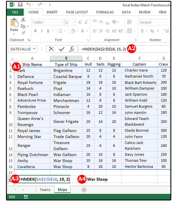
2. Enter the INDEX function (preceded by the equal sign), plus an
opening parenthesis, then highlight (or type) the database/table range
like this: =INDEX(A2:I16
Note: If you want an absolute reference (which, in this case, means
hard-coding the formula so when/if it’s copied, the range is not
altered), press F4 once after each cell reference. You could also
highlight the range: Just press F4 once after you select the full range,
and the complete absolute reference symbols are added.
3. Next, enter a comma to separate the arguments (that is, the
separate formula pieces); then enter the row number and a comma,
followed by the column number (yes, it must be a number and not the
usual column letter) and the right parenthesis (or just press Enter and
let Excel add the ending parenthesis for you). The complete formula
looks like this: =INDEX($A$2:$I$16,15,2).
Note: The row numbering starts with the first number in the range,
not the first number on the spreadsheet. For example, even though the
Cavalleria pirate ship is on Excel row 16, it’s actually row 15 in our
formula because our range begins on A2 and goes through I16. If A2 is
row 1, then A16 is row 15).
4. Note that the type of ship Norrington was looking for is a War Sloop. JD Sartain
Use the index function to locate specific information in your database.
B. INDEX ranges
Now, we can do lots more with this database table. You don’t need to
redefine the range every time you want to know something. To make it
easy, we’ll define the range one time and then name it. Then we can just
put the name of the range in our formulas.
1. Go to A2 and highlight the range A2 through I16.
2. From the Formulas tab, select Define Name from the Defined Names group.
3. In the popup dialog box, enter a name for your range in the Name field box.
4. Next, enter the Scope (where the range is located), which is either the Workbook or one of the worksheets in the Workbook.
5. Enter a comment, if necessary.
6. And last, verify that the Refers To field displays the correct name and range, then click OK.
7. If you’d like to verify that your range is, indeed, saved in
Excel, try this little test: Press Ctrl+G (the GoTo command). Select Ships in the GoTo dialog, then click OK, and Excel re-highlights the range A2:I16. How to define and save a range
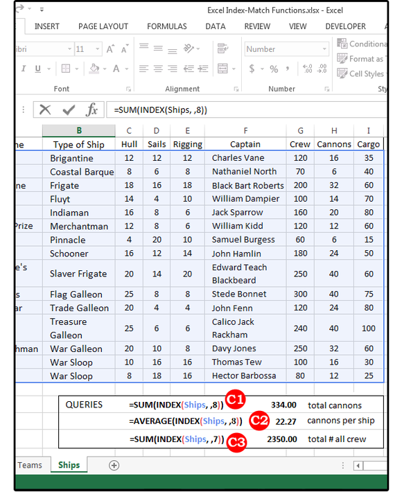
C. INDEX with SUM & AVERAGE formulas
Norrington is assessing the fleet’s battle capabilities. First he
wants to know how many cannons the pirates have, the average number of
cannons per ship, and the total number of crew manning all those pirate
ships. He enters the following formulas:
1. =SUM(INDEX(Ships, ,8)) equals 334, the total number of cannons, and
2. =AVERAGE(INDEX(Ships, ,8)) equals 22.27, or approximately 22.27 cannons per ship.
3. =SUM(INDEX(Ships, ,7)) equals 2350, the total number of all crew on all ships.
Why is there a comma, space, comma between Ships and the number 8,
and what do these numbers mean? Ships is the Range (followed by a
comma), the Row argument is blank (or a space) because Norrington wants
all rows, and the 8 represents the 8th column over (which is column H,
Cannons).
Some might ask, why not just enter the SUM and/or AVERAGE formulas at
the bottom of those columns? In this tiny spreadsheet, yes, it would be
just as easy. But if the spreadsheet has 5000 rows and 300 columns,
you’ll want to use INDEX JD Sartain
03 INDEX formulas using SUM and AVERAGE.
Once the range is named, Norrington can open a blank spreadsheet in
this same workbook and write his queries (formulas) in column B (which
show the results instead of the formulas) with a description that
defines those queries in column A. (Note: Column C shows the actual
formulas that are in column B).
He doesn’t have to visually see his huge database of 5000 records or
wait for several seconds while the formulas calculate. He can get all
the information he needs from his Query Sheet. Remember, the bigger the
spreadsheet, the slower it functions, especially if there are a lot of
formulas. JD Sartain
04 Commodore James Norrington’s pirate ship information / query sheet.
D. INDEX MATCH with MAX
Now, Norrington wants to know how many pirates are on the most
populated ship, and which ship is it? He uses the INDEX with MAX formula
to get the highest number of pirates, but he also needs to know which
ship is carrying them. So he uses the INDEX/MATCH with MAX formula to
find out which ship has the most pirates on board.
1. =MAX(INDEX(Ships, ,7)) equals 300, the highest number of pirates on one of the ships
2. =INDEX($A$2:$A$16, MATCH(MAX(Ships), $G$2:G$16, 0)) equals the Royal James, the ship with the most pirates aboard
3. =INDEX($F$2:$F$16, MATCH(MAX(Ships), $G$2:G$16, 0)) equals Stede Bonnet, Captain of the Royal James with a pirate crew of 300 JD Sartain
Use INDEX-MATCH and MAX to retrieve specific info from your database.


 The Find and Replace dialog box.
 Open the Quick Analysis panel by clicking its icon. Then choose a category heading and click an icon for a command.
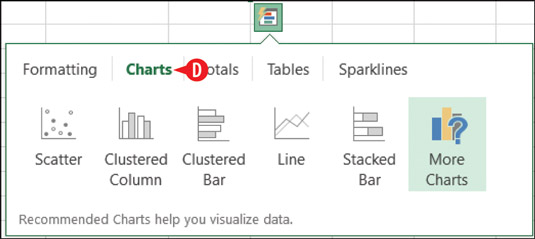 Quick Analysis offers shortcuts for creating several common chart types.
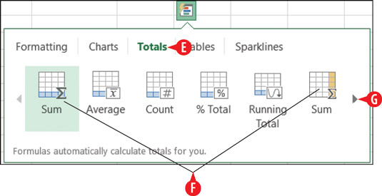 You can use Quick Analysis to add summary rows or columns.
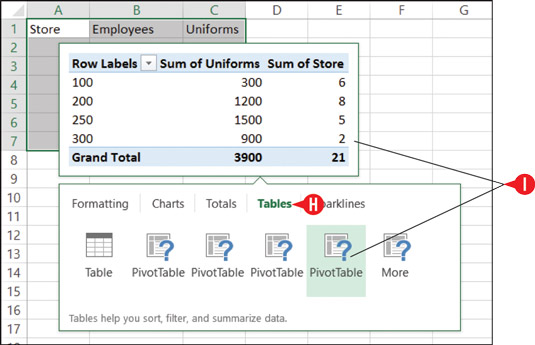 You can convert the range to a table or apply one of several PivotTable specifications.
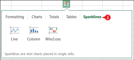 Choose Sparklines to add mini-charts that show overall trends.


 JD Sartain
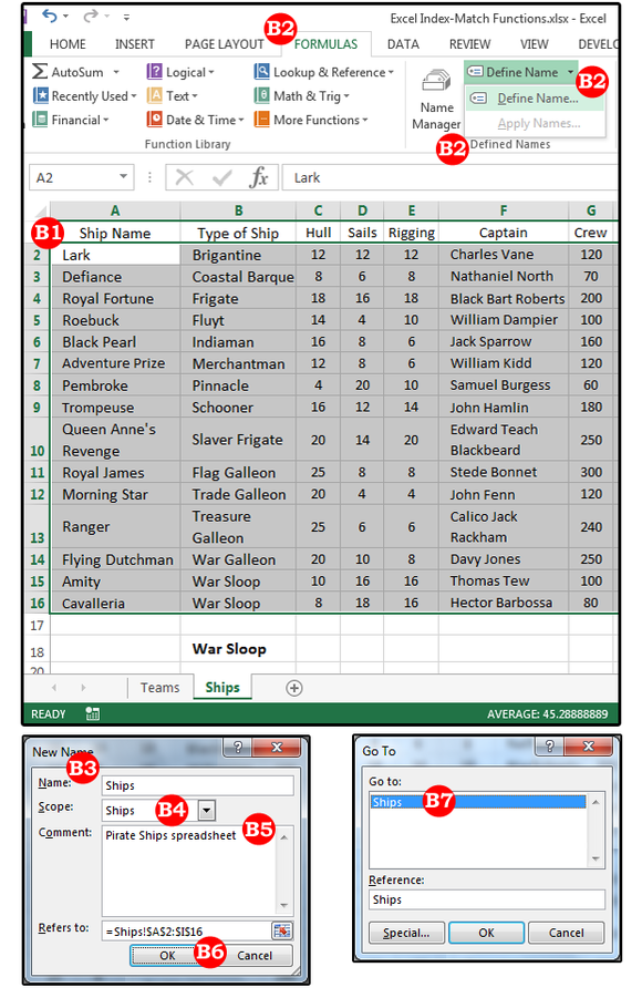
 JD Sartain
 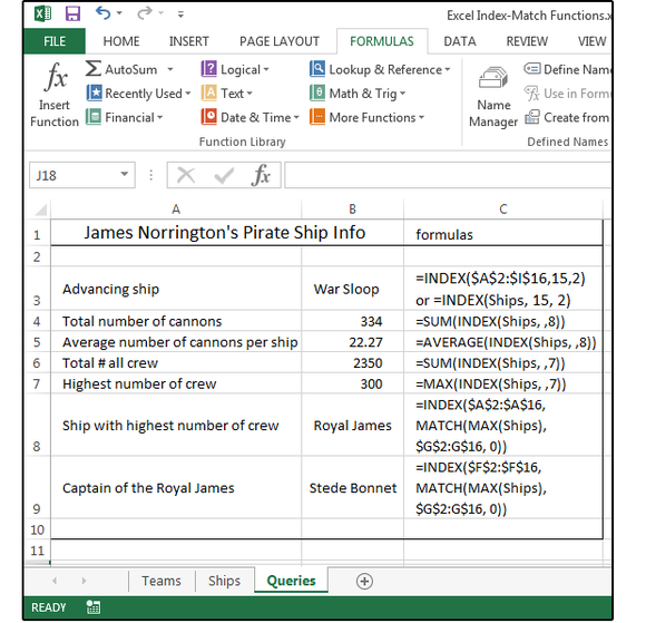 JD Sartain
 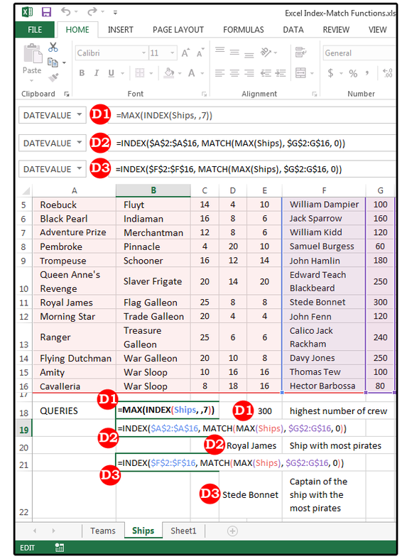 JD Sartain
  JD Sartain
 JD Sartain
  JD Sartain
  JD Sartain