
Drop-down lists are very useful data entry tools we see just about everywhere, and you can add custom drop-down lists to your own Excel worksheets. It’s easy and we’ll show you how.
Drop-down lists make it easier and more efficient to enter data into your spreadsheets. Simply click the arrow and select an option. You can add drop-down lists to cells in Excel containing options such as Yes and No, Male and Female, or any other custom list of options.
To begin, enter the list of age ranges into sequential cells down a column or across a row. We entered our age ranges into cells A9 through A13 on the same worksheet, as shown below. You can also add your list of options to a different worksheet in the same workbook.

Now, we’re going to name our range of cells to make it easier to add them to the drop-down list. To do this, select all the cells containing the drop-down list items and then enter a name for the cell range into the Name box above the grid. We named our cell range Age.

Now, select the cell into which you want to add a drop-down list and click the “Data” tab.

In the Data Tools section of the Data tab, click the “Data Validation” button.

The Data Validation dialog box displays. On the Settings tab, select “List” from the Allow drop-down list (see, drop-down lists are everywhere!).

Now, we’re going to use the name we assigned to the range of cells containing the options for our drop-down list. Enter
=Age
in the “Source” box (if you named your cell range something else,
replace “Age” with that name). Make sure the “In-cell dropdown” box is
checked.The “Ignore blank” check box is checked by default. This means that the user can select the cell and then deselect the cell without selecting an item. If you want to require the user to select an option from the drop-down list, uncheck the Ignore blank check box.

You can add a popup message that displays when the cell containing the drop-down list is selected. To do this, click the “Input Message” tab on the Data Validation dialog box. Make sure the “Show input message when the cell is selected” box is checked. Enter a Title and an Input message and then click the “OK” button.

When the cell containing the drop-down list is selected, you’ll see a down arrow button to the right of the cell. If you added an input message, it displays below the cell. The down arrow button only displays when the cell is selected.
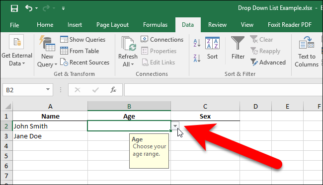
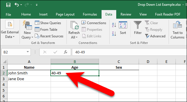
Click the down arrow button to drop down the list of options and select one.

If you decide you want to remove the drop-down list from the cell, open the Data Validation dialog box as described earlier and click the “Clear All” button, which is available no matter which tab is selected on the dialog box.

The options on the Data Validation dialog box are reset to their defaults. Click “OK” to remove the drop-down list and restore the cell to its default format.

If there was an option selected when you removed the drop-down list, the cell is populated with the value of that option.
Source: https://www.howtogeek.com/290104/how-to-add-a-drop-down-list-to-a-cell-in-excel/