This Excel Function Is So Much Smarter Than VLOOKUP

VLOOKUP has frustrated me with its rigid limitations and clunky syntax. But, not anymore. I found an Excel fucntion that handles lookups in any direction and offers precise matching control.

XMATCH Works in Any Direction You Want

The biggest frustration with VLOOKUP is its stubborn left-to-right requirement. If your lookup column isn't the leftmost in your range, you're stuck. You have to either rearrange your data or find a workaround. It can waste time restructuring spreadsheets just to make VLOOKUP happy.

Excel's XMATCH function eliminates this headache. Unlike VLOOKUP's rigid structure, XMATCH searches any array in any direction. You can find data to the left of your lookup column. You can also search vertically down a column or horizontally across a row; XMATCH handles both effortlessly.

Here's the basic syntax:

=XMATCH(lookup_value, lookup_array, [match_mode], [search_mode])

Let's break down these parameters:

• lookup_value: What you're searching for.
• lookup_array: The range where you're searching.
• match_mode: How exact your match needs to be (0 for exact, -1 for exact or next smallest, 1 for exact or next largest).
• search_mode: Which direction to search (1 for first to last, -1 for last to first, 2 for binary search).

Here's a practical example from an employee database. Say you need to find which department "Kristen Tate" works in, but the employee names are in column D while departments are in column B. With VLOOKUP in an Excel spreadsheet, this setup would force you to rearrange your data since you can't look left.

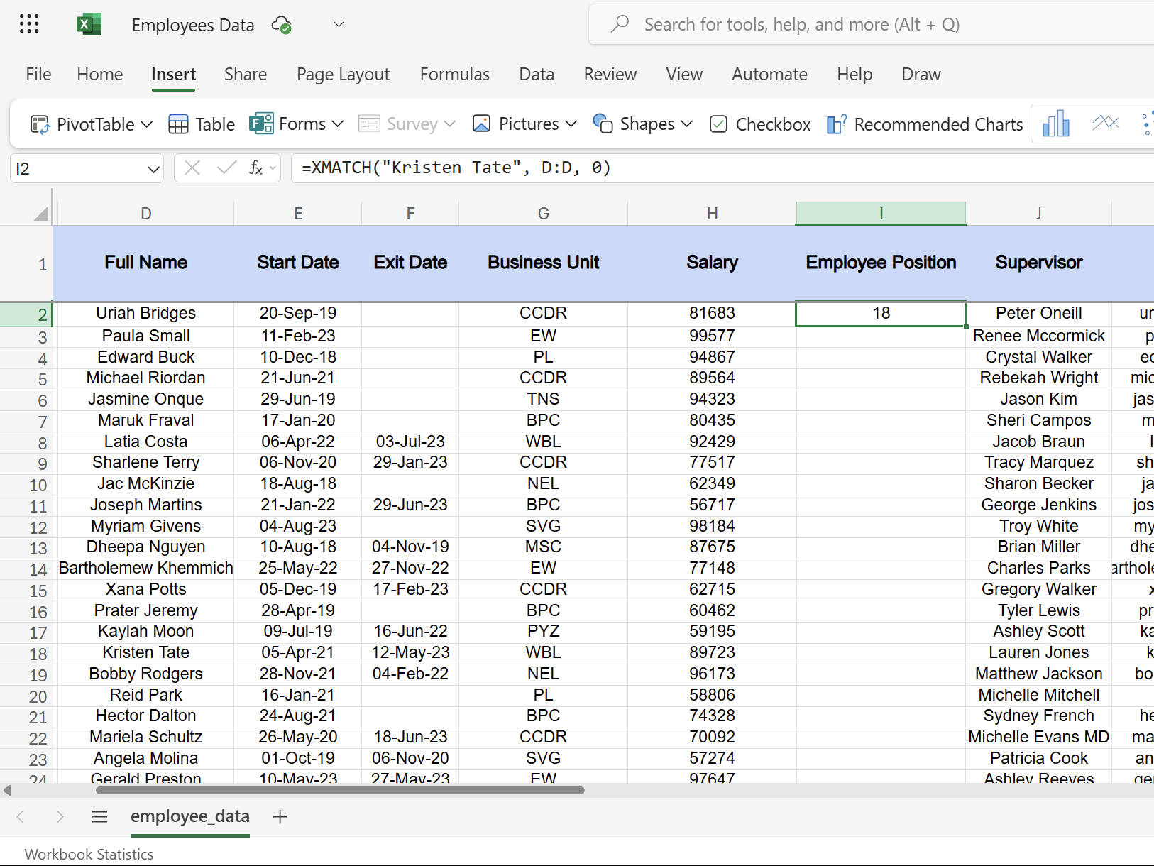
But you can use the XMATCH function to return her position in the name column as shown in the following formula:

=XMATCH("Kristen Tate", D:D, 0)

It changed my workflow as I no longer need to count columns. With VLOOKUP in an Excel spreadsheet, you're constantly counting to determine the column index number. If you add a new column to your data, suddenly your formulas break because the index numbers shift.

XMATCH Gives You Better Control Over Matching

VLOOKUP's matching options are limited to an exact match or an approximate match—that's it. If your data isn't perfectly clean, you're stuck spending time tidying up a messy Excel sheet before you can even start your lookup.

XMATCH makes it easy with its match_mode parameter. Set it to 0 for exact matches, just like VLOOKUP's FALSE parameter. But here's where it gets interesting. You can use -1 to find the exact match or the next smallest value, and 1 for the exact match or next largest value.

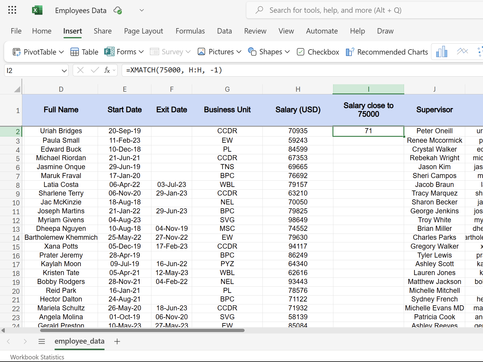
Consider salaries in the employee dataset. To find the employee earning closest to but not exceeding $75,000, you'd use:

=XMATCH(75000, H:H, -1)

This formula returns the position of the highest salary from column H that doesn't exceed your target value—something VLOOKUP struggles with unless your data is perfectly sorted.

The search_mode parameter adds another layer of control. While 1 searches from first to last (the default), -1 searches from last to first. This parameter matters when you have duplicate values and need the most recent entry.

For instance, if "John Smith" appears multiple times in column D of a dataset, we can use the following formula to find his last occurrence.

=XMATCH("John Smith", D:D, 0, -1)

Understanding these parameters helps you approach data lookup more effectively. This level of control means fewer helper columns and less data manipulation. Your formulas become more robust and your spreadsheets stay cleaner.

XMATCH Pairs Perfectly With INDEX

XMATCH proves more handy when you combine it with the INDEX function. While XMATCH finds the position, INDEX retrieves the actual value from that position. It's one of the useful Excel functions to find data quickly, but together, they create a more flexible lookup combination.

Here's the basic syntax when you combine both:

=INDEX(return_array, XMATCH(lookup_value, lookup_array, [match_mode]))

This pairing eliminates VLOOKUP's column-counting nightmare. Instead of remembering that salary is the eighth column, you simply specify the salary column directly. Hence, you don't get the broken formulas when you add or remove columns.

Let's say you need to find Kristen Tate's department from the employee data with INDEX and XMATCH:

=INDEX(R:R, XMATCH("Kristen Tate", D:D, 0))

The above formula reads naturally and returns a value from column R at the position where "Kristen Tate" appears in column D.

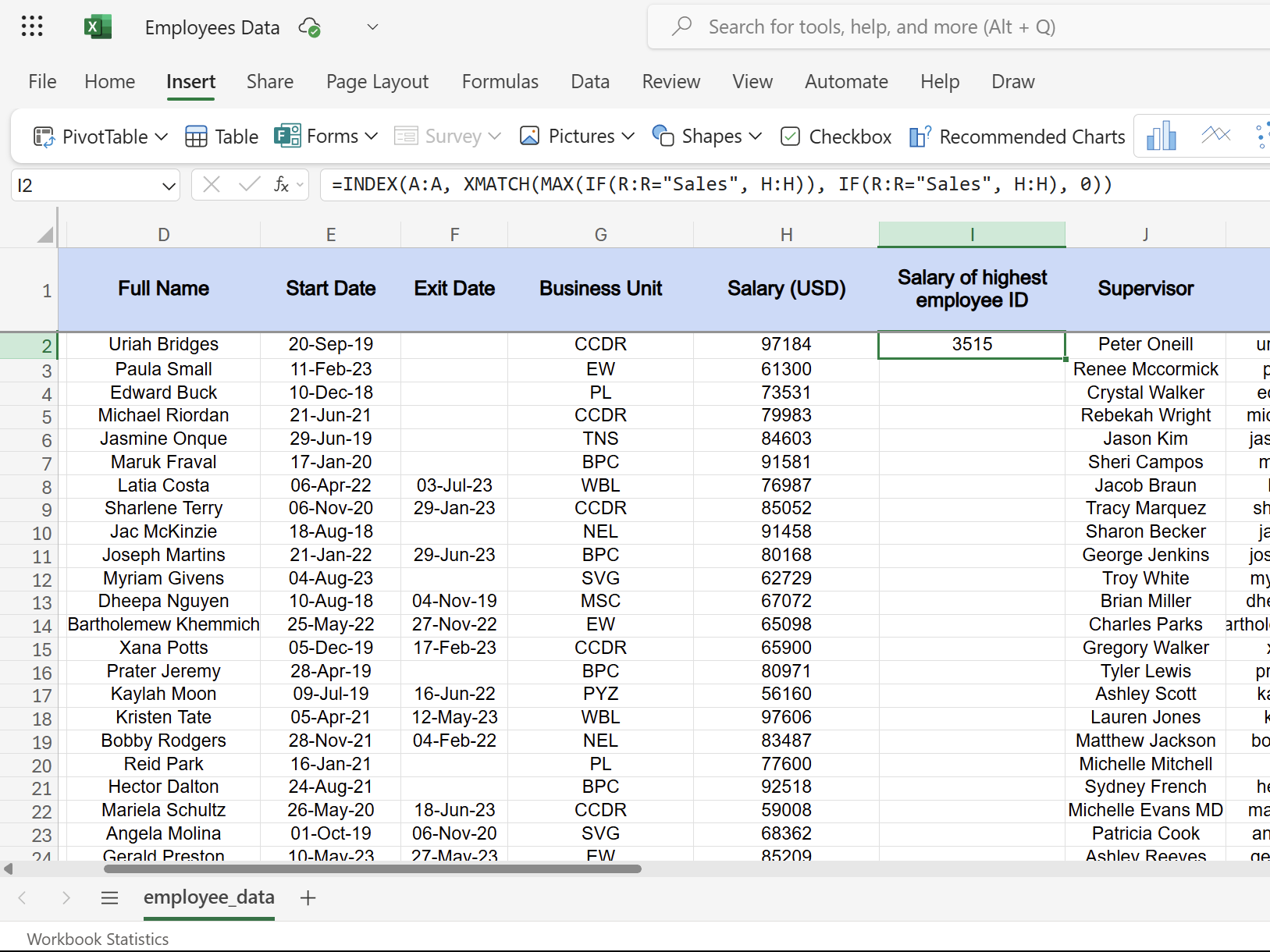
This combination also handles complex lookups, such as when you need the salary of the employee in the Sales department with the highest employee ID:

=INDEX(A:A, XMATCH(MAX(IF(R:R="Sales", H:H)), IF(R:R="Sales", H:H), 0))

This array formula finds the maximum employee ID within Sales, then returns that person's salary. If you were to try that with VLOOKUP, you'd need multiple helper columns and other workarounds.

XMATCH has completely replaced VLOOKUP in my workflow. The directional flexibility, precise matching control, and easy INDEX integration make it the lookup function that I needed the most. Once you experience this level of control, going back to VLOOKUP doesn't sound practical.

Source: https://www.makeuseof.com/xmatch-excel-function-vs-vlookup/

Here's the Easy Way to Insert a Table of Contents in Microsoft Word

A table of contents is incredibly useful, especially in long documents, as it eliminates the need to scroll through numerous pages to find the information you need. Thankfully, Microsoft Word makes inserting a table of contents into your document easy.

How to Create a Table of Contents Automatically in Word

Microsoft Word can automatically create a table of contents (TOC) based on the headings in your document. To use this feature, you first need to apply Word’s built-in heading styles to the headings and subheadings in your document.

To create headings, select the text, go to the Home tab, and choose the appropriate heading style from the Styles group. For example, use Heading 1 for main headings, Heading 2 for subheadings, and so on.

Once you've finished creating headings, follow these steps to insert a table of contents into your Word document.

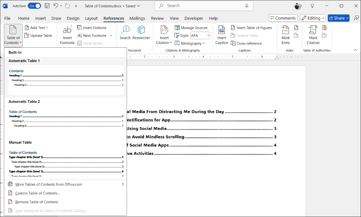
1. In your Word document, place the cursor where you want to insert the table of contents.
2. Switch to the References tab.
3. Click Table of Contents.
4. Select Automatic Table 1 or Automatic Table 2 from the menu.

Word will create and insert the table of contents at the specified location. You can then navigate to a heading quickly by holding the CTRL key and clicking on the entry you want to jump to.

If you want to remove the table of contents from your document, simply go to References > Table of Contents and select Remove Table of Contents.

How to Update the Table of Contents in Word

While Word makes it easy to create TOCs, it doesn't automatically update them when you edit headings or move them to different pages. Fortunately, updating the table of contents manually is straightforward. Here's how to do it:

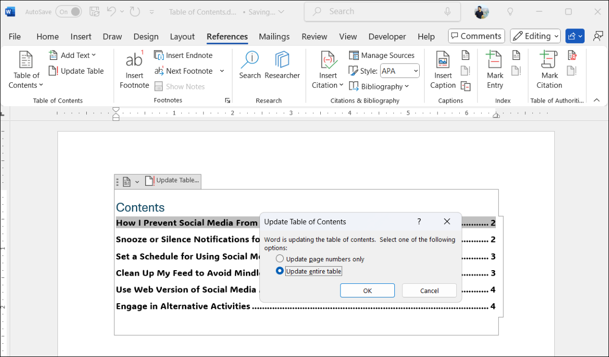
1. Click anywhere within the table of contents to select it.
2. Click the Update Table button that appears.
3. Choose Update page numbers only if you have only made changes that affect the page numbers.
4. Select Update entire table if you want to update the entire table of contents, including the headings.
5. Hit OK to confirm.

Your table of contents will now be updated to reflect the latest changes in your Word document.

How to Customize the Style and Appearance of Your Table of Contents

If Word's default table of contents feels too plain, don't worry. Word offers several customization options to help you tailor it to match your document's design. Here's how you can make your table of contents more visually appealing:

1. In your Word document, go to the References tab.
2. Click Table of Contents and select Custom Table of Contents.
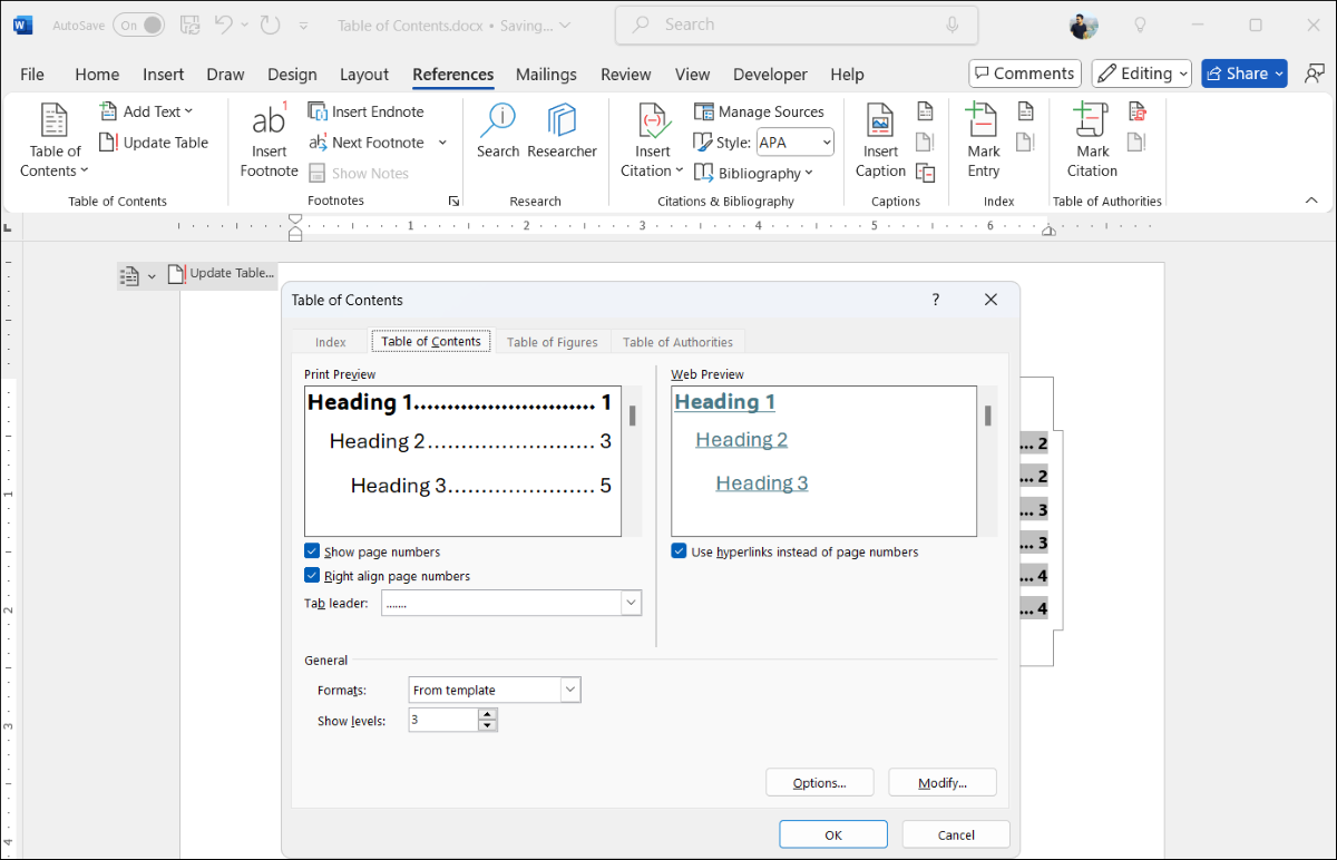
3. In the Print Preview section, use the checkboxes to show or hide page numbers and adjust the alignment. You can also change the pattern style between the heading title and the page number.
4. Under the General section, you can select from predefined styles and specify the number of heading levels you want to display in your TOC.
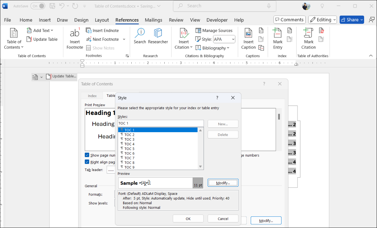
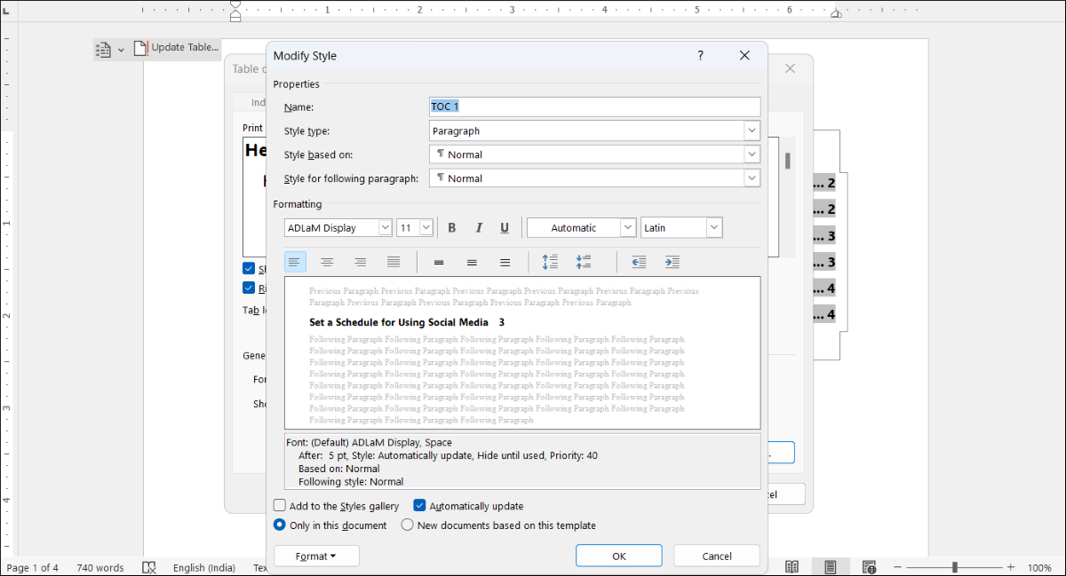
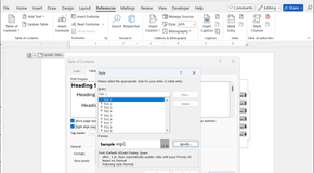
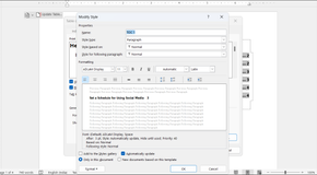
5. Click Modify to change the appearance of items in the table of contents. In the Styles list, select the level you want to change, and then click Modify to change the font, size, color, format, and more.
6. Once you’re done making the changes, click OK.

• 
• 
• 

• 
• 
• 

You can be as creative as you like while modifying the table of contents. If you need inspiration, check out these table of contents template examples for Microsoft Word. If customizing the table of contents manually seems like a lot of work, you can also download free, ready-made templates from the web.

Whether you choose to create a table of contents manually or use a template, it shouldn't take much time once you become familiar with the process.

Source: https://www.makeuseof.com/insert-table-of-contents-word/?utm_medium=newsletter&utm_campaign=MUO-202506100800&utm_source=MUO-NL&user=amltLm5hZ3kyQGdtYWlsLmNvbQ&lctg=02f46df6687a5c6b6c6a51453f460af32dc1bbe4d7321e3d7b193ec97761583e

How to Add a Drop-Down List to a Cell in Excel

Drop-down lists are very useful data entry tools we see just about everywhere, and you can add custom drop-down lists to your own Excel worksheets. It’s easy and we’ll show you how.
Drop-down lists make it easier and more efficient to enter data into your spreadsheets. Simply click the arrow and select an option. You can add drop-down lists to cells in Excel containing options such as Yes and No, Male and Female, or any other custom list of options.

It’s easy to add a drop-down list to a cell in Excel, but the process is not intuitive. Drop-down lists are created using the Data Validation feature. We’re going to create a drop-down list with a selection of age ranges to show you how it’s done.
To begin, enter the list of age ranges into sequential cells down a column or across a row. We entered our age ranges into cells A9 through A13 on the same worksheet, as shown below. You can also add your list of options to a different worksheet in the same workbook.





Now, we’re going to name our range of cells to make it easier to add them to the drop-down list. To do this, select all the cells containing the drop-down list items and then enter a name for the cell range into the Name box above the grid. We named our cell range Age.





Now, select the cell into which you want to add a drop-down list and click the “Data” tab.





In the Data Tools section of the Data tab, click the “Data Validation” button.





The Data Validation dialog box displays. On the Settings tab, select “List” from the Allow drop-down list (see, drop-down lists are everywhere!).





Now, we’re going to use the name we assigned to the range of cells containing the options for our drop-down list. Enter =Age in the “Source” box (if you named your cell range something else, replace “Age” with that name). Make sure the “In-cell dropdown” box is checked.
The “Ignore blank” check box is checked by default. This means that the user can select the cell and then deselect the cell without selecting an item. If you want to require the user to select an option from the drop-down list, uncheck the Ignore blank check box.





You can add a popup message that displays when the cell containing the drop-down list is selected. To do this, click the “Input Message” tab on the Data Validation dialog box. Make sure the “Show input message when the cell is selected” box is checked. Enter a Title and an Input message and then click the “OK” button.





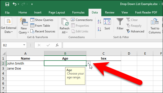
When the cell containing the drop-down list is selected, you’ll see a down arrow button to the right of the cell. If you added an input message, it displays below the cell. The down arrow button only displays when the cell is selected.





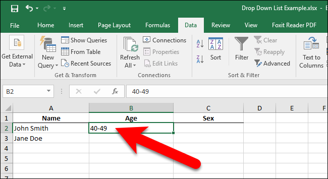
Click the down arrow button to drop down the list of options and select one.





If you decide you want to remove the drop-down list from the cell, open the Data Validation dialog box as described earlier and click the “Clear All” button, which is available no matter which tab is selected on the dialog box.





The options on the Data Validation dialog box are reset to their defaults. Click “OK” to remove the drop-down list and restore the cell to its default format.





If there was an option selected when you removed the drop-down list, the cell is populated with the value of that option.






Source: https://www.howtogeek.com/290104/how-to-add-a-drop-down-list-to-a-cell-in-excel/

How to Compare Two Columns in Excel: 7 Methods

 When working with large Excel spreadsheets, comparing the data from two columns can be time-consuming. Instead of analyzing the columns and writing “Match” or “Mismatch” into a separate column, you can use Excel’s functions to streamline the process.

We’ll take a look at how to use different Excel functions to compare two columns and identify matching or mismatching data.

1. How to Highlight Duplicate Data

If you want to compare two columns in Excel, but don’t want to add a third column showing if the data exists in both columns, you can use the Conditional formatting feature.

1. Select the data cells you want to compare.
2. Head to the Home tab.
3. From the Styles group, open the Conditional Formatting menu.
4. Click Highlight Cells Rules > Duplicate Values.

    

   

   5. In the Duplicate Values window, make sure the Format cells that contain option is set to Duplicate and choose the formatting option next to values with.
5. Click OK.

Excel will now highlight the names that are present in both columns.

2. How to Highlight Unique Data

You can use the same function if you want to identify data that isn’t part of both columns.

1. Select the data set.
2. Once again, head to Home > Conditional Formatting > Highlight Cells Rules > Duplicate Values.
3. For Format cells that contain, choose Unique.
4. Select how the mismatched data should be highlighted and click OK.

Excel will now highlight the names that can be found only in one of the two columns.

 

While these methods are quite easy to use, they might not be efficient for larger spreadsheets, so you’ll have to take think about an efficient way to organize your spreadsheet. So we’ll take a look at more complex solutions that show you which rows have the same data or use an additional column to display values indicating if the data matches or not.

3. Highlight Rows With Identical Data

If you need a better visual representation of identical data, you can make Excel find matching values in two columns and highlight the rows with matching data. As we did on the previous method, we’ll use the Conditional formatting feature, but will add a few extra steps.

This way, you will have a visual indicator that will help you identify matching data faster than reading through a separate column. Follow these steps to use Excel’s conditional formatting to compare two sets of data:

1. Select the data you want to compare (don’t include the headers) and open the Home tab.
2. Click Conditional Formatting and select New Rule.
3. From Select a Rule Type, click Use a formula to determine which cells to format.
4. Enter =$A2=$B2 into the field below Format values where this formula is true. Here, A and B correspond to the two columns we are comparing.

    

   

   5. To customize how Excel will highlight the rows, click Format, and in the Format cells window, select the Fill tab. You can choose the background color, pattern style, and pattern color. You will get a sample, so you can preview the design. Click OK once you’ve completed the customization process.
   
   
5. Click OK in the New Formatting Rule window, so Excel will highlight the rows with matching data instantly.

 

When comparing two columns in Excel using this method, you can also highlight the rows with different data. Go through the above steps, and at step 5, enter the =$A2<>$B2 formula within the Format values where this formula is true field.

4. Identify Matches With TRUE or FALSE

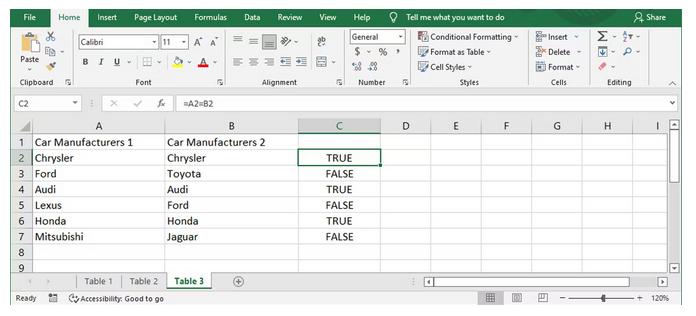
You can add a new column when comparing two Excel columns. Using this method, you will add a third column that will display TRUE if the data matches and FALSE if the data doesn’t match.

For the third column, use the =A2=B2 formula to compare the first two columns. If you think your spreadsheet will look too crowded with the TRUE and FALSE rows, you can set a filter in Excel, so it will only show the TRUE values.

5. Compare Two Columns With an IF Function

A different method to analyze Excel data from two columns is to use an IF function. This is similar to the above method, but it comes with the advantage that you can customize the displayed value.

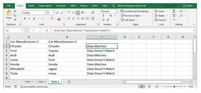
Instead of having the TRUE or FALSE values, you can set the value for matching or different data. For this example, we’ll use the Data matches and Data doesn’t match values.

The formula we’ll use for the column showing the results is =IF(A2=B2,"Data Matches","Data Doesn’t Match").

6. Compare Two Columns With a VLOOKUP Function and Find Matching Data

Another way to have Excel find duplicates in two columns is to use a VLOOKUP function. Excel will compare each cell in the second column against the cells in the first column.

Use the =VLOOKUP(B2,$A$2:$A$14,1,0) for the column displaying the results. Just make sure you adjust the data range.

 

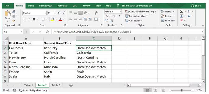
When using this formula, Excel will display the matching data or use a #N/A value. However, the #N/Avalue might be confusing, especially if you send the spreadsheet to someone else. If they are not experienced when it comes to Excel, they could believe there’s a mistake.


So to avoid any confusion, upgrade the VLOOKUP function to an IFERROR function. If you need to find data that is in column B and is also in column A, use the =IFERROR(VLOOKUP(B2,$A$2:$A$14,1,0),"Data Doesn't Match") formula.

This is just an example of a VLOOKUP function that you could use to search spreadsheets efficiently.

7. How to Compare Two Columns and Extract Data

Besides comparing two Excel columns for matches, you can also use the VLOOKUP function to extract matching data. This will save you time as you don’t have to manually go through the first column and search for relevant data.

Also, if data in the second column misses from the first column, Excel will display a #N/A value. For this, use the =VLOOKUP(D2,$A$2:$B$14,2,0) formula.

 

Note: If you want to protect your results from spelling mistakes, use the =VLOOKUP("*"&D2&"*",$A$2:$B$14,2,0) formula. Here, the asterisk (*) has the role of a wild card character, replacing any number of characters. This is just one of the ways you could use a wild card for better results in Excel

Compare Excel Columns With Ease

As we’ve discussed, there are plenty of ways and tricks you can use to compare two columns in an Excel spreadsheet and get the best results. You can even add a third column to display the results. You can even use Excel to compare physical documents, as you can quickly import data in Excel with its built-in tools.

Source: https://www.makeuseof.com/search/?q=How+to+Compare+Two+Columns+in+Excel%3A+7+Methods