Saturday, July 28, 2018

How to Create a Flowchart in Excel

Plenty of options exist for creating flowcharts, but you may not need one if you’re already subscribed to Microsoft Office 365. We’ve shown how you can create a flowchart in Word, but Excel works just as well.
In this article, we’ll show you how to set up a flowchart environment and create awesome flowcharts in Excel. We’ll end with some links where you can download free Microsoft Excel flowchart templates.


Set Up a Flowchart Grid in Excel

When creating a flowchart in Excel, the worksheet grid provides a useful way to position and size your flowchart elements.

Create a Grid

To create a grid, we need to change the width of all the columns to be equal to the default row height. The worksheet will look like graph paper.
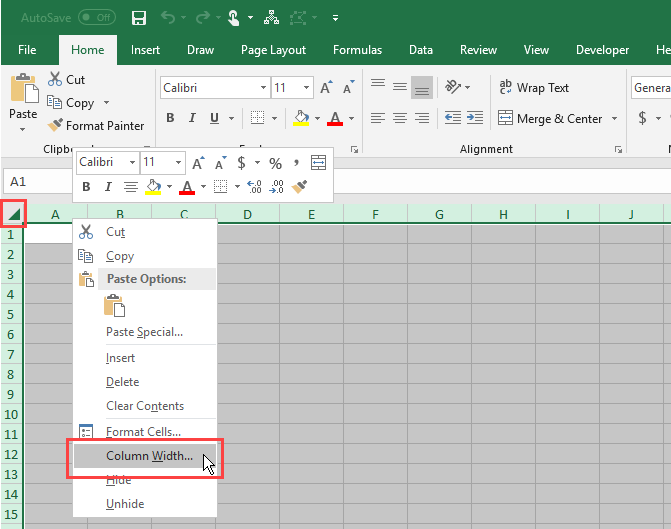
First, select all the cells on the worksheet by clicking the box in the upper-left corner of the worksheet grid. Then, right-click on any column heading and select Column Width.


Select all cells, then select Column Width in Excel
I


f you’re using the default font (Calibri, size 11), the default row height is 15 points, which equals 20 pixels. To make the column width the same 20 pixels, we must change it to 2.14.
So enter 2.14 in the box on the Column Width dialog box and click OK.
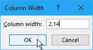
Change Column Width in Excel

Enable Snap to Grid

The Snap to Grid features makes it easy to place and resize shapes on the grid so you can consistently resize them and align them to each other. Shapes snap to the nearest grid line when you resize and move them.
Click the Page Layout tab. Then, click Align in the Arrange section and select Snap to Grid. The Snap to Grid icon on the menu is highlighted with a gray box when the feature is on.


Enable Snap to Grid in Excel

Set Up the Page Layout in Excel

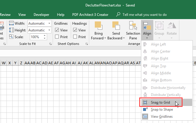
You should set up the page layout for your flowchart so you know your boundaries before laying out your flowchart. For example, if you’re going to insert your flowchart into a Word document, you should set the margins in Microsoft Excel to the same margins as your Word document. That way you won’t create a flowchart larger than the pages in your Word document.
To set up items like margins, page orientation, and page size, click the Page Layout tab. Use the buttons in the Page Setup section to change settings for the different layout options.


Change Page Orientation in Excel


How to Create a Flowchart in Excel

Now that your worksheet is set up for flowcharts, let’s create one.

Add a Shape Using the Shapes Tool

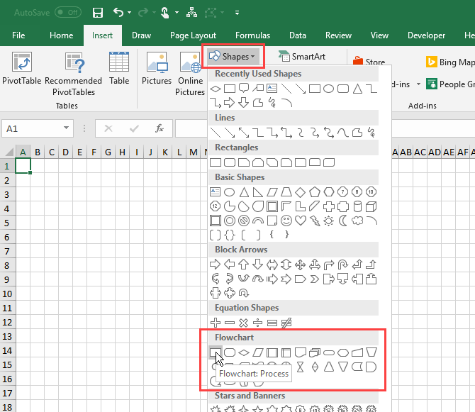
To add your first shape to your flowchart, go to the Insert tab and click Shapes in the Illustrations section. A dropdown menu displays a gallery of various types of shapes like basic shapes, lines, and arrows.
Select a shape in the Flowchart section of the dropdown menu.


Select a Shape in Excel


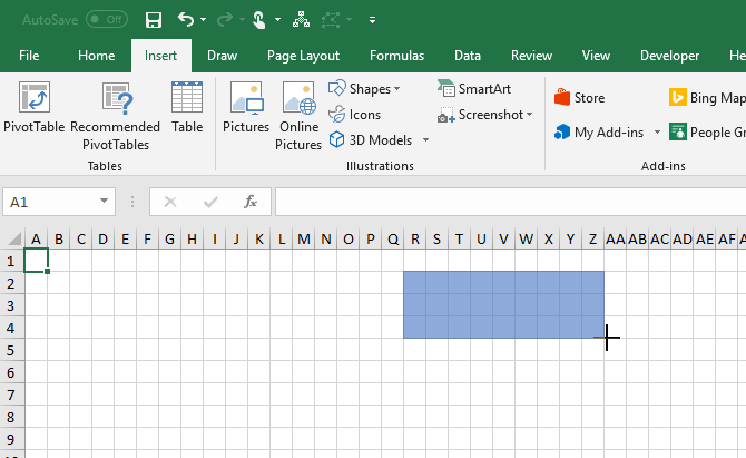
Drag the shape to the size you want on the worksheet. If Snap to Grid is enabled, the shape automatically snaps to the gridlines as you draw it.


Draw a shape on the grid in Excel


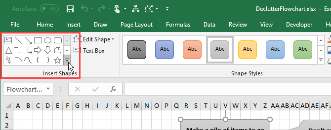
Add More Flowchart Shapes Using the Format Tab


Once you draw your first shape and select it, a special Format tab becomes available. You can use this tab to add more shapes to your flowchart and to format your shapes, which we’ll cover later.
A dropdown gallery of shapes displays, just like when you clicked Shapes in the Illustrations section on the Insert tab. Select the shape you want to add and draw it on the worksheet.
You can also double-click a shape on the gallery menu to add it to the worksheet. To resize the shape, select it and drag one of the handles along the edges.
To move the shape, move the cursor over the shape until the cursor becomes a cross with arrows. Then, click and drag the shape to where you want it.


Open the Shapes gallery on the Format tab in Excel

Add Text to a Shape

To add text to a shape, simply select the shape and start typing. We’ll show you later how to format the text and change its alignment.
To edit text in a shape, click on the text in the shape. This puts you in edit mode allowing you to add, change, or delete the text.
Click outside the shape or select the shape like you were going to move it as we talked about in the previous section.


Type text in a shape in Excel


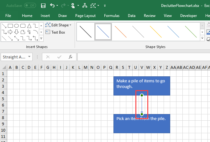
Add Connector Lines Between Shapes

After adding some shapes to your flowchart, it’s time to connect them.
Select Line Arrow on the shapes gallery either on the Insert tab or the Format tab.


Select Line Arrow in Excel


The cursor becomes a plus icon. Move the cursor over the first shape you want to connect. You’ll see dots at the points that represent connection points for that shape.
Click on the connection point where you want the line to start and drag the line to the next shape until you see the connection points on that one. Release the mouse on one of those points.
An arrow displays where the line ends. When a line is properly connected to a shape, the connection point is solid. If you see a hollow connection point, the line didn’t connect to the shape.


Draw a connector line on a flowchart in Excel

Add Text to Connector Lines

In flowchart programs like Visio and Lucidchart, you can add text directly to connector lines. In Microsoft Excel, you can’t do that. But you can do the next best thing.
2 Free Open Source Microsoft Visio Alternatives 2 Free Open Source Microsoft Visio Alternatives Need to create diagrams, flowcharts, circuits, or other kinds of entity-relationship models? Microsoft Visio is the best software for that, but it's expensive. We will show you two free open source alternatives. Read More
To add text to a connector line, you create a text box and position it along the line or on the line.
Select a shape or a connector line to activate the Format tab. Click the tab and then click Text Box in the Insert Shapes section.


Click Text Box in Excel


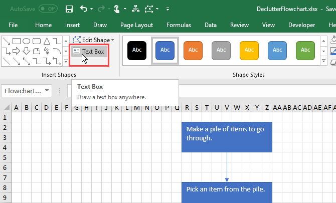
Draw the text box near the connector you want to label. Move the text box to where you want it the same way you move shapes.
You may want to turn off Snap to Grid when positioning text boxes on connector lines. This allows you to fine tune the size and position of the text boxes.
To add text, select the text box and start typing. We’ll show you how to format and position text boxes a bit later.


Add a text box near a connector line on a flowchart in Excel


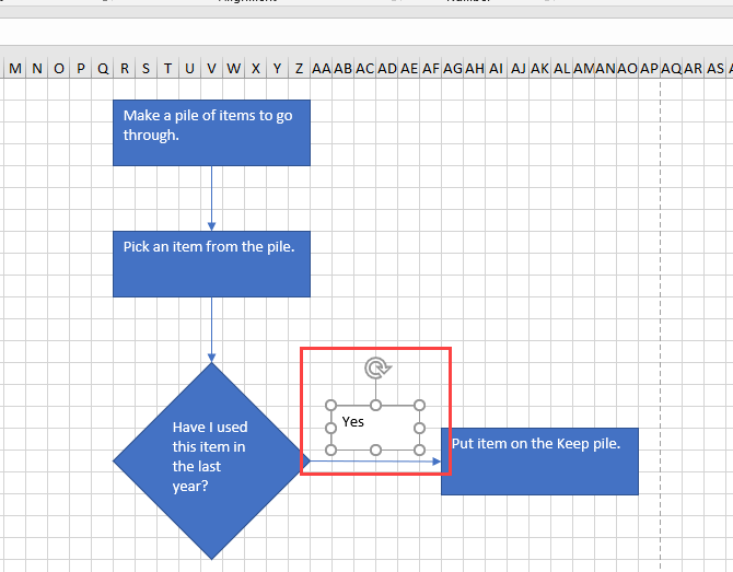
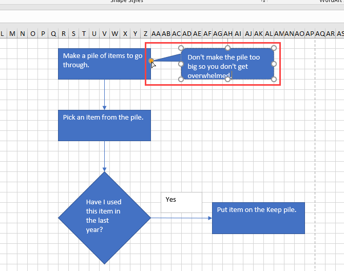
Add Notes Using Callouts

You can also use text boxes to add notes to your flowchart the same way you used them to add text to connector lines. And you can use a connector line to point to the area relating to the note.
But, that might be confusing and look like a step in the flowchart. To make a note look different, use a callout.
Select a callout from the shapes gallery either on the Insert tab or the Format tab.


Select a callout shape in Excel


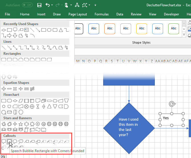
Draw the callout on the worksheet just like you would draw a shape.
Add text to the callout and use the handles to resize it the same way you would on a shape.
Initially, the part of the callout that points shows on the bottom border. To make the callout point to where you want, click and drag the point. When the point connects with a shape, the connection point turns red.


Draw a callout in Excel


How to Format a Flowchart in Excel

Excel has many formatting options, too many to cover here. But we’ll show you a few basics so you can format your shapes, text, and connector lines.
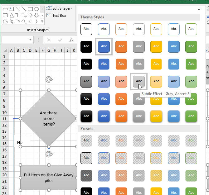
Format Shapes

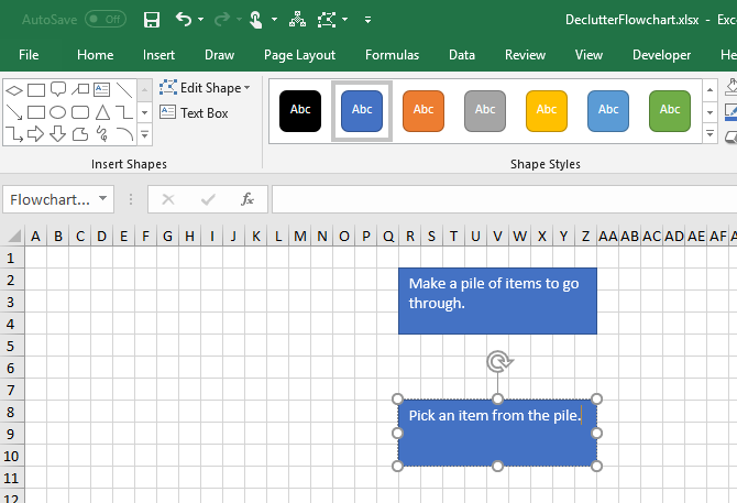
An easy way to format shapes and the text in shapes is to use Theme Styles.
Select all the shapes you want to format with the same style. Click on the first shape, then press and hold down Shift while clicking the other shapes. Then, click the Format tab.
Click the More arrow in the lower-right corner of the Theme Styles box in the Shape Styles section. A gallery of styles displays in a dropdown menu.
When you move your mouse over the various theme styles, you’ll see how they look on your shapes. Click the style you want to use.


Change the Theme Style for shapes in Excel


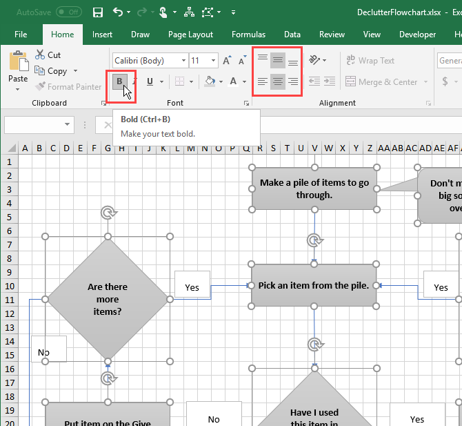
Format Text in the Shapes and Text Boxes

Formatting text in shapes and text boxes is done the same way you normally format text in cells.
First, we’ll format shapes. Select all the shapes containing text you want to format using the Shift key while clicking the remaining shapes after the first one.
Click the Home tab and use the commands in the Font and Alignment sections to format your text. For example, we used the Center and Middle Align buttons in the Alignmentsection to center the text in the shapes horizontally and vertically. Then, we applied Boldto all the text.
Do the same thing with the text boxes along the connector lines to format and align the text.


Format text in shapes using the Home tab in Excel

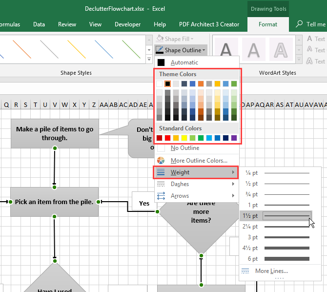
Format Connector Lines

The default format on the connector lines is a bit thin. We’re going to make them thicker.
Select all the connector lines you want to format using the Shift key while clicking the remaining lines after the first one. Then, click the Format tab.
Click Shape Outline in the Shape Styles section and select a color from the Theme Colors section or Standard Colors section. Then, on the same menu, go to Weight and select a thickness for the connector lines from the submenu.


Change color and weight for connector lines on a flowchart in Excel


Get Started With These Excel Flowchart Templates

Excel flowchart templates provide a quick start when creating your own flowcharts. We’ve previously covered flowchart templates for Microsoft Office, but these are specifically for Microsoft Excel.
Here are more templates you can download:


Organize Your Life With Excel Flowcharts!

The ability to create flowcharts in Microsoft Excel makes it a very useful and versatile tool for keeping yourself organized. It’s not the only option, though. There are several good free flowchart tools available for Windows.
7 Best Free Flowchart Tools for Windows 7 Best Free Flowchart Tools for WindowsFlowcharts can help you streamline your work and life and break free from bad habits. But what's the best way to make a flowchart? We've found 7 great flowchart tools. Read More

Source: https://www.makeuseof.com/tag/create-flowchart-excel/

Saturday, July 21, 2018

How to create simple and dependent drop-down lists

Using tables, named ranges, formulas, data validation, and table styles

Drop-down lists in Microsoft Excel (and Word and Access) allow you to create a list of valid choices that you or others can select for a given field. This is especially useful for fields that require specific information; fields that have long or complex data that’s hard to spell; or fields where you want to control the responses.
Creating dependent drop-down lists (when combined with an INDIRECT function) is another benefit. This allows you to select a product category from the main menu drop-down list box (such as Beverages), then display all the related products from the submenu (dependent) drop-down list box (such as Apple Juice, Coffee, etc.). This works very well for ordering and inventory purposes because it divides all the products into manageable categories. This is how most wholesale and retail companies handle their product lines. In fact, companies from hospitals and insurance carriers to banks and more use drop-down lists, check boxes, combo lists, and/or radio buttons to minimize typing and user errors.

How to create a simple drop-down list

We’ve created a sample drop-down list so you can practice the steps, or feel free to use your own data.

If your spreadsheet database is large or contains numerous fields, we recommend that you place the list box items in a table on a separate spreadsheet, but in the same workbook. However, if your list is relatively short, you can type the items for your list, separated by commas, in the Source field of the Data Validation dialog window.
1. Open a new workbook and add a second spreadsheet tab (click the ‘+’ sign at the bottom of the screen on the tab bar).
2. Rename Spreadsheet 1 as “wks” for worksheet, and Spreadsheet 2 as “lists.”
3. Enter the names of 10 doctors (or other applicable items) in column A from A1 through A10.
4. Sort the list to your preference. If you plan to sort by last name, enter the last name first, then the first name and middle initial on your original list.
5. Highlight the range (A1:A10) or just position your cursor on any cell in the list, and press Ctrl+ T to convert this group of items to a table. Excel calls it Table 1, 2, 3, etc., which is not a problem if there is only one table. Be sure to check the box that says “My Table Has Headers.”
Note: When data is in a table, you can add or delete items from the list (and all other drop-down lists that use that same table) and they will all update automatically.


01 enter your list of items then convert the list to a table JD Sartain / IDG Worldwide


Enter your list of items, then convert the list to a table.
6. Move to Spreadsheet 1 (renamed wks). Enter some data similar to that shown in the following graphic, for example: Type of Surgery, Date, Time, and Surgeon, or create your own data.
7. Select the cell or group of cells where you want the drop-down list to appear. In this case, select D2 (or D2:D11, if you prefer, though it's not necessary to highlight the entire column).
8. From the Data tab, select Data Validation > Data Validation.
9. In the Data Validation dialog window, choose the Settings tab. In the Validation Criteria panel in the Allow field, select the option called List from the drop-down list box.


02 from the settings tab choose list from the list box JD Sartain / IDG Worldwide


From the Settings tab, choose List from the list box.
10. Tab down to the Source field and click inside this box.
11. Move your cursor outside of this dialog window and select the lists spreadsheet from the workbook tabs at the bottom of the screen.
12. Highlight the range of doctors—that is, A2 through A11. Notice that Excel adds this range in the Source field box (=lists!$A$2:$A$11) for you.
13. Next, click the Input Message tab and enter a Title and Input Message for your drop-down list.
14. Next, click the Error Alert tab and enter the Title and Error Message for your drop-down list.
15. Click OK and your drop-down list box is complete.


03 enter the source range input message error alerts JD Sartain / IDG Worldwide


Enter the Source range, Input Message, and Error Alerts for your drop-down list box.
16. Move back to the wks spreadsheet and position your cursor in cell D2. Notice the arrow for the drop-down list box, and your custom Input Message appears to the right of each cell in this column that you select. Click the down arrow and choose a doctor from the list that specializes in the type of surgery on the corresponding row of column A. For example, Dr. Simon Walters’ field is hip surgery.
17. If anyone types an invalid name—that is, they try to type in a name that is not on the Acceptable Surgeon’s list, the custom error message that you specified appears when the Enter key is pressed. Click Cancel to exit this dialog.


04 choose a doctor or type an invalid entry for error alert JD Sartain / IDG Worldwide


Choose a doctor from the list or type an invalid entry for an Error Alert.
Create dependent drop-down lists
Dependent drop-down lists are like the submenus in Office applications. The main menu (or drop-down list) displays various options with submenus below each one that display further options related to the main menu. In our sample worksheet, the drop-down list provides a selection of surgeons for you to choose that matches the type of surgery scheduled.
For this next exercise, imagine that you run a small rural hospital located about 50 miles from a large city that has three large, completely staffed hospitals. It’s your job to schedule surgeons from one of these three large facilities to see patients at your hospital. The “main” drop-down list contains a selection of hospitals (by location) where each surgeon practices. The submenu drop-down lists provide the names of each surgeon that works in each of these facilities: East Side, West Side, or Midtown.

A. Create the lists

1. First, add another spreadsheet and name it lists2.
2. On the lists2 spreadsheet, enter the following title for column A: Hospital Locations. Under Hospital Locations enter the names EastSideWestSide, and Midtown in cells A2, A3, and A4, respectively (without spaces or use one word).
3. Move your cursor to the first cell under the title Hospital Locations (A2). Click Home > Format As Table, and choose a Table Style from the submenu, then click OK.
4. Select the hospital locations in this list (A2:A4). Enter a table name (Locations) in the Name box (above column A) or press Ctrl+ T to convert these items to a table, which Excel names Table 1, 2, 3, etc. Finally, check the box that says My Table Has Headers.
5. To rename your tables, select Formulas > Name Manager. Cursor down to Table 1 (2, 3, 4, etc.), then click the Edit button.
6. In the Edit Name dialog box, type in the new name (Locations).
Note: Excel does not allow spaces or other special characters. Names must begin with a letter or an underscore, and names cannot conflict with any of Excel’s built-in names or other objects in the workbook (for instance, you cannot have two ranges with the same name in a single workbook—even if the ranges are in separate spreadsheets).


05 rename your tables using excels name manager JD Sartain / IDG Worldwide

Rename your tables using Excel’s Name manager.
7. Next, you must create a separate table for each of the hospital locations. On the lists2 spreadsheet, enter the following titles, for column B: East Side, C: West Side, and D: Midtown (these column labels will also be your range names minus the spaces).
8. Enter some doctors' names under each of these three columns (B, C, D).
9. Format each list as a named table (repeat step 3 above).
10. Highlight the range of each column individually (B1:B8; C1:C7; D1:D9). Press Ctrl+ T to convert these groups of items to Tables, which Excel names Table 2, 3, 4, etc., then check the box that says My Table Has Headers. Repeat steps 5 and 6 above to rename your tables. Remember, no spaces in range names.


06 create tables for your lists JD Sartain / IDG Worldwide

Create tables for your lists.
Note: If you have multiple tables, name them based on the header you provided for each column.

B. Create the drop-downs

1. First, return to the wks spreadsheet and delete the previous drop-down list in column D titled Surgeons. Create a new header in column D1 titled Location, and name column E1 Surgeons.
2. Select cells D1:E11, then select Home > Format As Table, choose a style, check the headers box, and click OK.
3. Next, select cells (D2:D11) for the main menu drop-down list.
4. From the Data tab, select Data Validation > Data Validation.
5. In the Data Validation dialog window, choose the Settings tab. In the Validation Criteria panel in the Allow field, select the option called List from the drop-down list box.
6. In the Source box, click the list2 spreadsheet, highlight the Hospital Location list minus the header (A2:A4), and click OK.


07 create the main menu dropdown list JD Sartain / IDG Worldwide

Create the main menu drop-down list.

7. Move your cursor to cell E2.
8. Repeat steps 8 and 9 above.
9. This time, in the Source box, enter this formula: =INDIRECT($D$2)—but this is for the current cell only—then click OK.
Note: If you receive the Source Error message, just click Yes, because the errors will cease when the data from the drop-down lists fill in.
10. To fill out the column (which is the obvious course), enter the formula like this: =INDIRECT($D2)—yes, without the '$' sign on the row number—then copy cell D2 down from D3 through D11. This activates the entire range.

08 enter the indirect function as a relative formula then copy JD Sartain / IDG Worldwide

Enter the INDIRECT function as a relative formula, then copy.
11. If you want to add an Input Message or an Error Alert, repeat steps 13 through 14 above in the section "How to create a simple drop-down List."

C. Test your work

Now it’s time to test your work. Click the drop-down arrows (one at a time) in column D (Location).
1. Choose a hospital from the list, and it appears in the active cell.
2. Move your cursor to column E (Surgeon) and choose a doctor from the list of doctors at the location you specified in column D.

09 the drop down lists work as expected JD Sartain / IDG Worldwide


The drop-down lists work as expected.

D. Work-around for two word items

If you want to use two or more words for the main menu drop-down (e.g., Location) and you do not want to run the words together without a space (e.g., East Side instead of EastSide), enter this formula in the dependent drop-down (Surgeon) Source box in the Data Validation dialog window:

=INDIRECT(SUBSTITUTE(D2," ","")) where D2 is the cell address, " " means quote-space-quote, and "" means quote-quote with no space. Translation: substitute cell D2 that has a space with D2 minus the space.
That’s all for now. If you need additional help, you can download this spreadsheet here:

Source: https://www.pcworld.com/article/3276341/office-software/excel-how-to-create-simple-and-dependent-drop-down-lists.html