Wednesday, October 15, 2014

How to Remove Duplicate Rows in Excel

When you are working with spreadsheets in Microsoft Excel and accidentally copy rows, or if you are making a composite spreadsheet of several others, you will encounter duplicate rows which you need to delete. This can be a very mindless, repetitive, time consuming task, but there are several tricks that make it simpler.

Getting Started

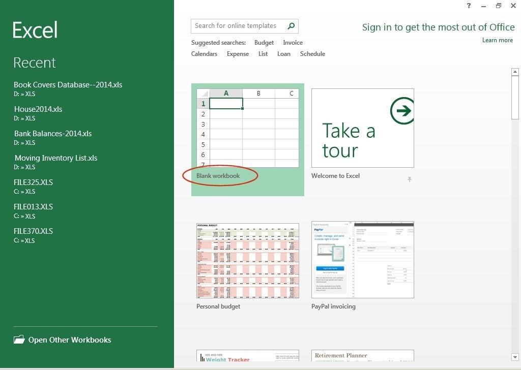
Today we will talk about a few handy methods for identifying and deleting duplicate rows in Excel. If you don’t have any files with duplicate rows now, feel free to download our handy resource with several duplicate rows created for this tutorial. Once you have downloaded and opened the resource, or opened your own document, you are ready to proceed.
Duplicate Rows 1

Option 1 – Remove Duplicates in Excel 2007 and 2010

If you are using Microsoft Office Suite 2007 or 2010 you will have a bit of an advantage because there is a built in feature for finding and deleting duplicates.
Begin by selecting the cells you want to target for your search. In this case, we will select the entire table by pressing “Control” and “A” at the same time (Ctrl + A).
Duplicate Rows 2
Once you have successfully selected the table, you will need to click on the “Data” tab on the top of the screen and then select the “Remove Duplicates” function as shown below.
Duplicate Rows 3
Once you have clicked on it, a small dialog box will appear. You will notice that the first row has automatically been deselected. The reason for this is that the “My data has headers” box is ticked.
Duplicate Rows 4
In this case, we do not have any headers since the table starts at “Row 1.” We will deselect the “My data has headers” box. Once you have done that, you will notice that the whole table has been highlighted again and the “Columns” section changed from “duplicates” to “Column A, B, and C.”
Duplicate Rows 5
Now that the entire table is selected, you just press the “OK” button to delete all duplicates. In this case, all the rows with duplicate information except for one have been deleted and the details of the deletion are displayed in the popup dialog box.
Duplicate Rows 6

Option 2 – Advanced Filtering in Excel 2007 and 2010

The second tool you can use in Excel to Identify and delete duplicates is the “Advanced Filter.” This method also applies to Excel 2003. Let us start again by opening up the Excel spreadsheet. In order to sort your spreadsheet, you will need to first select all using “Control” and “A” as shown earlier.
After selecting your table, simply click on the “Data” tab and in the “Sort & Filter” section, click on the “Advanced” button as shown below. If you are using excel 2003, click on the “Data” drop down menu then “Filters” then “Advanced Filters…”
Duplicate Rows 7
Now you will need to select the “Unique records only” check box.
Duplicate Rows 8
Once you click on “OK,” your document should have all duplicates except one removed. In this case, two were left because the first duplicates were found in row 1. This method automatically assumes that there are headers in your table. If you want the first row to be deleted, you will have to delete it manually in this case. If you actually had headers rather than duplicates in the first row, only one copy of the existing duplicates would have been left.
Duplicate Rows 9

Option 3 – Replace

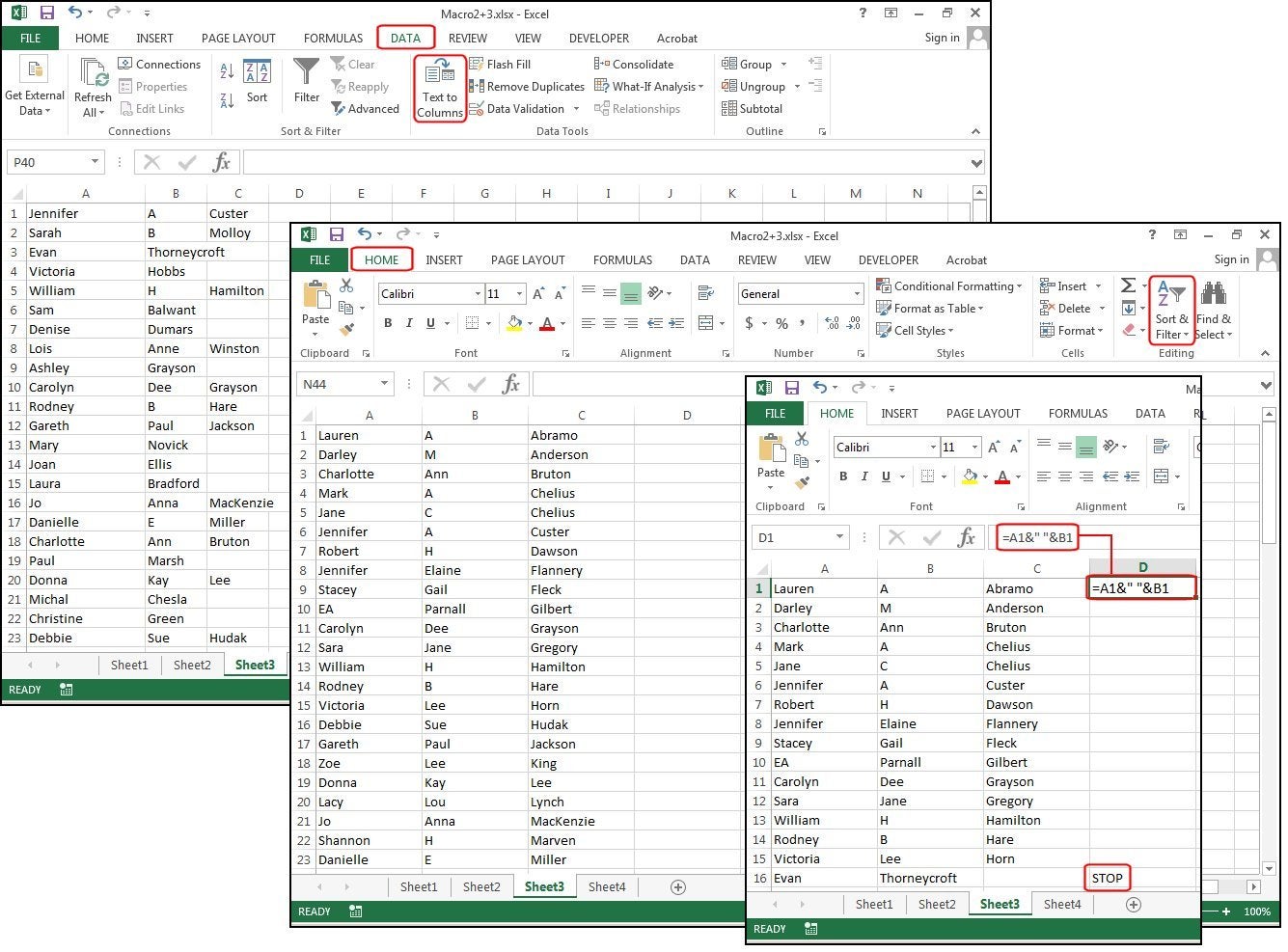
This method is great for smaller spreadsheets if you want to identify entire rows that are duplicated. In this case, we will be using the simple “replace” function that is built into all Microsoft Office products. You will need to begin by opening the spreadsheet you want to work on.
Once it is open, you need to select a cell with the content you want to find and replace and copy it. Click on the cell and press “Control” and “C” (Ctrl + C).
Duplicate Rows 10
Once you have copied the word you want to search for, you will need to press “Control” and “H” to bring up the replace function. Once it is up, you can paste the word you copied into the “Find what:” section by pressing “Control” and “V” (Ctrl + V).
Duplicate Rows 11
Now that you have identified what you are looking for, press the “Options>>” button. Select the “Match entire cell contents” checkbox. The reason for this is that sometimes your word may be present in other cells with other words. If you do not select this option, you could inadvertently end up deleting cells that you need to keep. Ensure that all the other settings match those shown in the image below.
Duplicate Rows 12
Now you will need to enter a value in the “Replace with:” box. For this example, we will use the number “1.” Once you have entered the value, press “Replace all.”
Duplicate Rows 13
You will notice that all the values that matched “dulpicate” have been changed to 1. The reason we used the number 1 is that it is small and stands out. Now you can easily identify which rows had duplicate content.
Duplicate Rows 14
In order to retain one copy of the duplicates, simply paste the original text back into the first row that has been replaced by 1’s.
Duplicate Rows 15
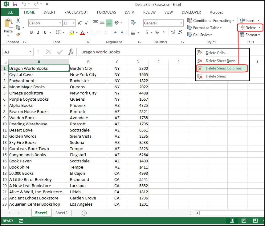
Now that you have identified all the rows with duplicate content, go through the document and hold the “Control” button down while clicking on the number of each duplicate row as shown below.
Duplicate Rows 16
Once you have selected all the rows that need to be deleted, right click on one of the grayed out numbers, and select the “Delete” option. The reason you need to do this instead of pressing the “delete” button on your computer is that it will delete the rows rather than just the content.
Duplicate Rows 17
Once you are done you will notice that all your remaining rows are unique values.
Duplicate Rows 18

Source: http://www.howtogeek.com/198052/how-to-remove-duplicate-rows-in-excel/

Thursday, September 11, 2014

5 must-know Excel macros for common tasks

If you’re not using macros, you’re ignoring one of Excel’s most powerful features. Macros save you time and spare you headaches by automating common, repetitive tasks. And you don’t have to be a programmer or know Visual Basic Applications (VBA) to write one. With Excel 2013, it's as simple as recording your keystrokes.
Here we’ll show you how to create macros for five commonly performed functions.

Macro Basics

To record a macro, click Record Macro under the Developer tab. In the Record Macro dialog box, enter the following information and click OK when you’re done.
Macro Name —the first character must be a letter, followed by your choice of letters, numbers, or an underscore. No other characters are accepted.
Shortcut Key —CTRL+J and CTRL+M are available. If you choose any other character, your macro will overwrite that key’s original function.
Save location —Macros saved in “This Workbook” or “New Workbook” function only in those workbooks. To use in all spreadsheets, save macros to the Personal Macro Workbook (PMW).
Description —Describe the macro.

f1 macrobasics
Name, save, and define your macro.
Because macros perform repetitive tasks, the object is to use them on a lot of different spreadsheets. This means you cannot hard-code the cell addresses (C1, D5, etc.), unless all of the spreadsheets are identical, which means the same number of records in the same columns and rows. To make the macro work on all spreadsheets with similar data, you must use the directional keys to navigate—then, the number of records won’t matter—and always begin at the A1 position.

Organize, format, and sort imported data

Data from other programs is often available in TSV or CSV files (Tab- or Comma-Separated Values). Imagine receiving two dozen of these files every month, which have to be organized, unwanted data removed, and then sorted by company name. It takes hours to do a report like that. This macro does it in seconds.
Open the CSV worksheet. Follow the directions above to name, define and save your macro, then record the keystrokes below.
1. Press CTRL+Home to reposition your cursor in cell A1. Hold down the CTRL key and click the letters over the columns you want to eliminate (B through N plus R). Select Home>Delete>Sheet Columns.

f2 delete unwanted columns
What a mess. First delete unwanted columns.
2. Hold down the CTRL key and click columns A and D. Select Home>Format>Column Width>42>OK. Hold down the CTRL key and click columns B and C. Select tab Home>Format>Column Width>25>OK.
3. Press CTRL+Home, then CTRL+A (to select all data in the spreadsheet).
Select Home>Sort & Filter>Custom Sort. In the Sort dialog box under Column, choose Name. Under Sort On, choose Values, and under Order, choose A-Z.
f3 sort
Sort by company name.
4. Select Developer>Stop Recording, and it’s finished. Save the worksheet as an Excel file. Open the CSV file again, select Developer>Macros, select the BranchCSV macro from the list, and click Run. The entire worksheet is organized in one second.
f4 run macro
Open the CSV file again and run the macro.

Split names from one column into two

How many times have you received a long list of names in one column you needed split into two columns, so the first and last name are separated? This macro does it in seconds plus sorts the list, adjusts the column widths, and gives a total list count. Open the Names worksheet, name and define your macro, then record these keystrokes.
1. Press CTRL+Home, CTRL+A. Select Data>Text to Columns. In the first Wizard dialog box, click Delimited>Next. In the second box, choose the character that delimits (separates) your text. Our list is separated by spaces, so check Space>Next. In the last box, click Text>Finish.
g1 text to column feature
Choose Text to Column to separate first and last names.
2. Press CTRL+Home, then CTRL+A. Select Home>Sort & Filter>Custom Sort. In the Sort dialog, select column B in the Sort By field. Click Add Level, then select column A in the Then By field. For Sort On and Order, leave the defaults Values and A-Z, then click OK.
g2 sortfilter
Sort two levels, last name, then first name.
3. Press CTRL+Home. Press Shift-Right-Arrow to highlight A1 thru B1. Click Format>Column Width>15>OK.
4. Press CTRL+Home. Select Home>Insert Sheet Rows, twice. In A1, type Total Names. Use the right arrow key to navigate to B1, then enter this formula: =COUNTA( and press CTRL+Down-Arrow, End, Shift-Down-Arrow, Enter, CTRL+Home. The total appears in B1.
g3 add formula run macro
Enter the formula to count the names in the list, then run the macro.
5. Stop Recording, save the worksheet as Names2. Open the Names file again and run the macro.

Split column and adjust for middle names

In Excel 2013, it’s easy to divide one column of names into two columns, but what if half the list contains middle names/initials and half does not? This macro extracts the middle names/initials entries, rejoins them with the first names, then produces one list with first/middle name in first column and last name in second column. Open a three-names file, name and define your macro, then record these keystrokes.
1. Press CTRL+Home, CTRL+A. Select Data>Text to Columns. In the Wizard boxes, click Delimited>Next, Space>Next, and Text >Finish. One column becomes three.
2. Press CTRL+Home, CTRL+A. Select Home>Sort & Filter>Custom Sort>column C. Press Shift-Right-Arrow. Click Format>Column Width>15>OK.
3. Press CTRL+Home, Right Arrow twice. Press End once, Down-Arrow twice, Right Arrow once—this moves the cursor to the first empty cell in column C, then to the adjacent cell in column D. Type: STOP, press Up Arrow, End, Up Arrow. Type this formula: =A1&” “&B1, then press Enter, Up Arrow.
p1 text columnsort width stop formula
Use directional keys to navigate so the macro works on all similar worksheets.
4. Press CTRL+C, Down-Arrow. Hold down Shift, then press End, Down Arrow, Up Arrow, Enter (copies formula). Press Up Arrow once, hold down Shift, press End, Down Arrow, Up Arrow (this highlights the range without STOP).
5. Press CTRL+C, CTRL+Home, select Paste>Paste Special>Values>OK. Press Escape, CTRL+Home, Right Arrow twice. Hold down Shift, press End, Down Arrow, CTRL+C, Left Arrow, Enter to copy last names. Press Right Arrow, Shift-Right-Arrow.
p2 copypaste formula delete columns
Copy and paste the formula, then remove extra columns.
6. Select Delete>Delete Sheet Columns. Press CTRL+Home. Stop Recording, save the worksheet as 3Names2; open 3Names again and run the macro.

Repetitive Text

If you’re typing the same information 10 times a day, you're begging for a macro. Even if that information is brief, a macro does it in seconds and ensures accuracy. This macro adds your company info to the top of a worksheet and inserts the current date. Open a new worksheet, name and define your macro, then record these keystrokes.
1. Press CTRL+Home. Hold down Shift, then Right Arrow twice. Select Home. From the Alignment group, select Merge Across. Enter this formula in cell A1: =TODAY() Enter, Up Arrow. Select Home>Format>Format Cells>Date. Choose a date format from the list, click OK. Press Down Arrow twice.
2. Type the repetitive information and press Enter at the end of each line. Press Down Arrow. Select Developer>Stop Recording. Delete it all, unmerge cells A1 through A3, then run the macro. Save the worksheet.
s1 repetitive text
Create a header macro with the current date to eliminate repetitive typing.

Remove Blank Rows

A worksheet filled with blank rows is impossible to manage, sort, or calculate. The first step is to instruct the macro to highlight the spreadsheet data only, then select and remove the blank rows. Once that’s accomplished, you can easily manage the data.
Open a file with blank rows, name and define your macro, then record these keystrokes.
1. Press CTRL+Home. Note: CTRL+A will not select all the data when blank rows are in the spreadsheet, but this macro will.
2. Select Home>Insert>Sheet Column. Press End, Down Arrow, Right Arrow, End, Up Arrow. Press CTRL+Shift-Home, Shift-Right-Arrow, CTRL+Shift-Right-Arrow. And the data range is properly selected.
s3 blanks removed
Remove blank rows.
3. Select Home>Find & Select>GoTo Special (or press CTRL+G, ALT+S). Click Blanks>OK and all the blanks highlight in gray. Select Delete>Delete Cells>Shift Cells Up>OK and the blanks vanish. Press CTRL+home, then select Delete>Delete Sheet Column to remove the extra column we inserted to highlight the spreadsheet without hardcoding cell addresses.
4. Stop Recording. Undo all steps, then run the macro. Save the worksheet.

Source: http://www.pcworld.com/article/2604739/5-must-know-excel-macros-for-common-tasks.html#tk.rss_all

Friday, May 30, 2014

Open Excel 2013 without a blank workbook


Tired of opening Excel from your desktop shortcut and seeing an empty workbook? Then follow these step-by-step instructions to create an application that will not display an empty workbook. 
Help users increase productivity by automatically signing up for TechRepublic's free Microsoft Office Suite newsletter, featuring Word, Excel, and Access tips, delivered each Wednesday.
If you normally launch Excel 2002 by clicking a shortcut on your desktop, you may not want to see an empty workbook. To prevent Excel from displaying an empty workbook when it is started, follow these steps:
  1. In Windows Explorer, go to \Program Files\Microsoft Office\Office10\Shortcut bar\Office and delete the existing shortcut for Excel. (In Excel 2003, go to \Program Files\Microsoft Office\Office11\Shortcut bar\Office.)
  2. In Windows Explorer, go to \Program Files\Microsoft Office\Office10. Then, right-click the EXCEL.exe icon and select Create Shortcut. (In Excel 2003, go to \Program Files\Microsoft Office\Office11. Then, right-click the EXCEL.exe icon and select Create Shortcut.)
  3. Right-click the shortcut icon and select Properties.
  4. In the Shortcut tab, add a space, followed by the /e switch to the path in the Target box. For example, in Excel 2002, the entry in the Target box would be: "C:\Program Files\Microsoft Office\Office10\EXCEL.exe" /e
  5. Click OK.
When you double-click the Excel shortcut icon, the application will open without displaying a blank workbook.

Source: http://www.techrepublic.com/article/open-excel-without-a-blank-workbook/

Thursday, May 29, 2014

How to create 3D Worksheets in Excel 2013

One of Excel’s greatest tricks is the dimensional or 3D reference. This feature, which allows you to create formulas that refer to the same cell or range on multiple worksheets, simplifies the creation of complex documents like monthly inventories or sales reports. In Excel 2013, Microsoft has beefed it up with enhanced options and formulas.
To illustrate the power and flexibility of 3D worksheets, we’ll create a Year-to-Date project that calculates the utility bills for a small business for each month, with the year-to-date totals on the first sheet. This workbook (which contains of all the worksheets in this project) calculates the columns, rows, and multiple spreadsheets three-dimensionally.
Because retyping the same data is counterproductive, we’ll create the month of January first, add the formulas for the columns and rows, and then copy this sheet 12 times (one for each month, plus the year-to-date sheet).
Start by selecting Blank workbook from the Home menu page.
f1 excelhomemenu blank workbook
In Excel 2013 Home Menu, select Blank workbook.

Sheet title and custom date

In cell A1, type January 2014. Excel changes the format to Jan-14. Right-click the mouse in that cell and choose Format Cells from the dropdown list. Choose Date from the format options, and you’ll notice that there is not a format listed for the month spelled out with a four-digit year. Choose Custom and in the Type field box above the list enter mmmm yyyy, then click OK. Now your title says 'January 2014.'
This small business has four designers who rent space. The rent is divided equally, but the utilities and other fees are calculated by percentages of use, therefore each designer pays a different price. Be sure to use the actual percent sign when you enter these numbers.

Enter data and format cells

In cells A4 through G4 enter this data: Total, Monthly, Carrie C, Marilyn H, Pat B, Donna A, and Percent Total. In cells A5 through G5 enter this data: Utilities, Totals, 28%, 32%, 17%, 23%, and Verified. Select cells A4 through G5 and click Center from the Ribbon bar on the Home menu tab. Note: You can center both horizontally and vertically.
In cells A6 through A15, enter this information: Electricity, Gas, Water, Garbage, Shop Phone, Internet, Alarm Service, Maintenance, Cleaning Services, TOTALS. Adjust column widths to fit the data entered. In B6 through B14, enter these numbers: 646, 510, 211, 56, 165, 98, 55, 335, and 400. Select cells B6 through G15, then click Center, and then click Increase Decimal (two times) to format for two decimal places (both on the Home menu tab).
f2 enter dataformat cells
Enter worksheet data and format the cells.

Add formulas

This part is really easy and, by copying all the formulas, really fast. In cell C6 enter this formula:
=sum(B6*C5) and click Enter. With your cursor on C6, press F2 to edit the formula. Position your cursor before the 'B' in 'B6' (between the left parenthesis and the B), then press F4 three times—until you see a dollar sign appear in front of the letter 'B.' Still in edit mode, move the cursor to the left of the letter C in C5 and press F4 twice (until you see a dollar sign appear in front of the number 5), then press Enter. Your formula in C6 should look like this: =sum($B6*C$5). This little trick locks the pieces of the formula (that is, column B and row 5) that you don’t want to change (called absolute reference) and therefore prevents lots of editing.

Copy formulas

Reposition your cursor to C6. Click Copy from the Ribbon bar (or press Ctrl+C). Move your cursor to C7, select cells C7 through C14, then press Enter. With C7 through C14 still selected, click Copy again, move your cursor to D7, select D7 through F14, then press Enter. All the cells will calculate.
Now, to verify that all the calculations are correct (in case there’s a typo somewhere), position the cursor in G6 and enter this formula: =sum(C6:F6) and press Enter (you can also highlight these ranges and let Excel fill in the cell locations). With your cursor on G6, click Copy, select cells G7 through G14, and press Enter. If the numbers in column G match the numbers in column B exactly, then your formulas are all correct.
Next, position your cursor on cell B15 and enter this formula: =sum(B6:B14) and press Enter. With your cursor on B15, click Copy, select cells C15 through G15, and press Enter.
f3 addcopy formulas
 Add and copy formulas to worksheet.

Copy and rename spreadsheets

f4 copy spreadsheets
Copy Spreadsheet 12 Times.
Copy this spreadsheet 12 times for a full year's worth of data. Place your cursor on the Sheet1 tab at the bottom of your Excel window. Right-click the mouse and select Move or Copy from the drop list. Check the box that says Create a Copy, select (move to end), then click OK.
Double-click the tab that says Sheet1 and rename it YTD. Double-click the remaining sheet tabs Sheet1 (2) through Sheet1 (12) and rename the worksheet tabs Jan, Feb, Mar, etc., through Dec. Next, change the titles of each sheet to match the tabs (type over 'January 2014' with correct titles). Note: Keep spreadsheet tab titles as short as possible for easier dimensional calculating.
f5 rename spreadsheets
Rename spreadsheets and spreadsheet tabs.
Access spreadsheets Feb through Dec and enter some random numbers in the Monthly Totals column—cells B6 through B14 (not B15, because it’s a formula). For this example, the dimensional totals only calculate Jan through May.

Add 3D worksheet formulas

On the YTD spreadsheet, position your cursor on B6 and enter this formula: =sum(Jan:Dec!B6). Copy this formula from B6 down to B7 through B14 (not B15, because this formula totals this column).
f6 addcopy 3d spreadsheet formulas
Add formulas to total spreadsheets dimensionally from Jan through Dec.
Next, select cells B6 through B14, select Copy, then highlight C6 through F14 and press Enter. The YTD spreadsheet now has the totals from the entire year. Every time you make a change in column B (Monthly Totals) on spreadsheets Jan through Dec—that is, every time you make an adjustment to the individual utility fees—the entire spreadsheet recalculates to reflect those new numbers.
f7 addcopy 3d spreadsheet formulas2
Copy dimensional formulas from column B to remaining columns in YTD spreadsheet.
In 2015, delete the numbers in column B from B6 thru B14 on all spreadsheets from Jan through Dec, then enter the correct utility fees each month as the bills arrive. Watch the YTD spreadsheet totals change as it adds each month's totals. Once these spreadsheets are created with the formulas, you’ll never have to repeat this process.

Future edits are easy

If you have to add or remove a utility from a 3D worksheet, be sure to stay inside the calculated area. For example, if the alarm service is discontinued in June of 2015, don’t change anything. Just enter zeros in that cell for July through Dec. Then, in January of 2016, place your cursor on that row (on each spreadsheet, Jan through Dec, including the YTD spreadsheet) and select Delete Sheet Row (from the Home menu tab).
To add a new utility, place your cursor anywhere between cells B6 and B14 and select Insert Sheet Row. Then copy the formulas for that row from the row above it. Inserting new rows inside the matrix ensures that the new row’s numbers and formulas are included in the project-wide formulas. If rows are inserted outside the matrix, the numbers and formulas on this row will not be included in any of your calculations unless you adjust all your formulas to include this new range.
Note that when you insert a new row between B6 and B14, the TOTALS row moves down to B16, and the formula in that cell (which totals column B) changes from =sum(B6:B14) to =sum(B6:B15). Stay inside the original matrix range, and everything will calculate accurately throughout the entire project.
f8 adddelete rows
Stay inside the original spreadsheet matrix when adding or deleting rows.


Source: http://www.pcworld.com/article/2241304/how-to-create-3d-worksheets-in-excel-2013.html#tk.rss_all

Wednesday, May 21, 2014

Excel 2013 tutorial: Creating PivotTables | lynda.com


Published on Feb 8, 2013
Find out how to create PivotTables to view and analyze data dynamically in Excel 2013. Watch more at http://www.lynda.com/Excel-tutorials/....

This tutorial is a single movie from the Excel 2013 Essential Training course presented by lynda.com author Dennis Taylor. The complete course duration is 6 hours and 8 minutes long and teaches you the basics of using Excel 2013 to enter and organize data, use functions, and build charts and PivotTables

1. Getting Started with Excel 2013
2. Entering Data
3. Creating Formulas and Functions
4. Formatting
5. Adjusting Worksheet Layout and Data
6. Printing
7. Introduction to Charting
8. Adjusting Worksheet Views
10. IF, VLOOKUP, and Power Functions
12. The Database Features of Excel
13. PivotTables
14. Data Analysis Tools
9. Multiple Worksheets and Workbooks
11. Security and Sharing
Introduction
15. Introduction to Macros
Conclusion


Source: http://www.youtube.com/watch?v=cLQ8A2889gk

Monday, April 7, 2014

Customize, Change Theme color, Default font in Office 2013

I have been using latest version of the Office for a few months now. It makes me share some tips, every time I discover something new with the productivity suite that I am not aware of. In this topic we shall learn to change theme and font of Office 2013 documents. Let’s get started!


If you intend to change your current theme, switch to a different one, or create a new theme, you may find the Design tab in Word or the Page Layout tab in Excel as the right place to start.

Change Theme color in Office 2013

First off, open a new document, choose the ‘Designs’ tab, click the drop-down arrow of ‘Colors’ and pick the color of your choice.


Pick Color Customize, Change Theme color, Default font in Office 2013


Now, if you would like to create your own set of colors, choose ‘Customize Colors’ option.
Next, from the customize colors window that opens up, click the button adjacent to the theme color of your choice (for example, Accent 1 or Hyperlink), and then pick a color under ‘Theme Colors’.


customize colors1 Customize, Change Theme color, Default font in Office 2013


For creating a customized or your own new color,  click ‘More Colors’ and pick a color on the Standard tab or enter numbers on the Custom tab.


Standard Colors Customize, Change Theme color, Default font in Office 2013
Source: http://www.thewindowsclub.com/change-theme-color-default-font-office