How to Perform a Two-Way Lookup in Excel With INDEX and XMATCH

For many, the INDEX-XMATCH combination in Excel is the go-to method for retrieving a value from a dataset. However, you can also use this dynamic duo to perform two-way lookups, returning a value at the intersection of a specified row and column.

This article is aimed at readers across all levels of Excel expertise, increasing in complexity as it progresses. If you're unfamiliar with the INDEX and XMATCH functions, continue reading. However, if you already know how to use INDEX and XMATCH for one-way lookups, jump straight to the section headed Using INDEX With XMATCH for Two-Way Lookups.

How Excel's INDEX and XMATCH Functions Work

Before we look at how these two functions can be used together in one formula, let's take a moment to explore how they work in isolation.

The INDEX Function

The INDEX function returns a value in a range according to the row number and column number you specify. The syntax is as follows:

=INDEX(a,b,c)

where

• a is the range,
• b is the row number, and
• c is the column number.

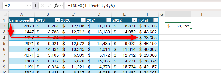
For example, typing:

=INDEX(T_Profit,3,6)

into cell H2 returns the value in the cell that sits at the intersection of the second row and the third column of the T_Profit table.



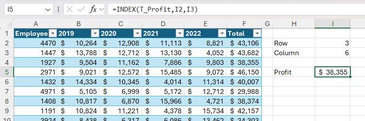
What's more, instead of hardcoding the row and column numbers, you can reference cells containing them, making the formula more flexible. Here, typing:

=INDEX(T_Profit,I2,I3)

into cell I5 pulls the row number from cell I2 and the column number from cell I3.



The XMATCH Function

The XMATCH function searches for an item in a range and returns its position.

If you're working in the Excel desktop app on a PC or Mac, you need to be using Excel 2021 or later (including Excel for Microsoft 365) to use the XMATCH function. It's also readily available in Excel for the web and on the Excel tablet and mobile apps.

Here's the syntax:

=XMATCH(a,b,c,d)

where

• a is the item to look up,
• b is the range to search,
• c is the match type (0 = exact match (default); -1 = exact match or next smallest item; 1 = exact match or next largest item; 2 = a wildcard match), and
• d is the search mode (1 = first to last (default), -1 = last to first, 2 = binary search where b is in ascending order, -2 = binary search where b is in descending order).

You may be familiar with the MATCH function, which is the predecessor to the more modern XMATCH function. They work in similar ways, though the default arguments in the XMATCH syntax are more intuitive than those in the MATCH syntax, favoring an exact match over an approximate one. Also, XMATCH lets you search in either direction and use wildcard characters for partial matches—both of which you can't do with MATCH.

In this example, typing:

=XMATCH(1927,T_Profit[Employee])

into cell H2 returns 3, because the employee ID number 1927 is the third value in the Employee column of the T_Profit table.



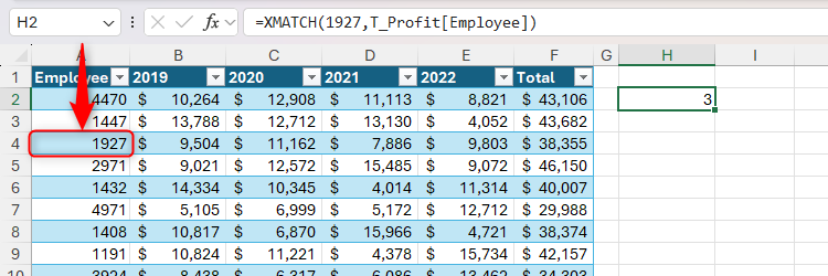
Notice how arguments c and d aren't required in this scenario, because we want an exact match in a search that runs from the top of the table to the bottom, and these are the default settings for this function.

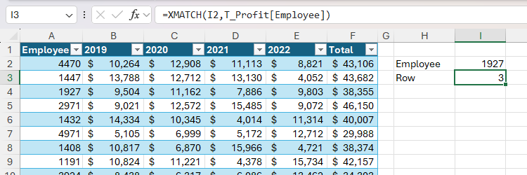
Similarly, argument a can be a reference to a cell containing the lookup value, meaning you can easily change the lookup value without editing the formula:

=XMATCH(I2,T_Profit[Employee])

where cell I2 contains the employee ID to look up in the Player column of the T_Scores table.



Using INDEX With XMATCH for One-Way Lookups

While the INDEX and XMATCH functions can be useful on their own, their true potential is realized when used together. The key to understanding how the INDEX-XMATCH combination can be used to perform two-way lookups is to first get your head around how it works in one-dimensional situations.

Let's say you want to view the total profit generated by an employee when you type their ID into cell I2.



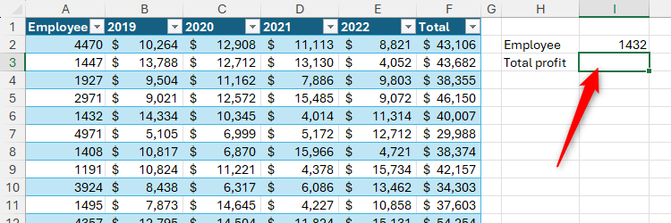
To do this, in cell I2, type:

=INDEX(T_Profit,XMATCH(I2,T_Profit[Employee]),6)

where

• T_Profit is the name of the table where the value will be found,
• XMATCH(I2,T_Profit[Employee]) tells the INDEX function which row of the Employee column to look in, based on the value in cell I2, and
• 6 tells the INDEX function to return the value in the sixth column of that row.

Instead of typing structured table references manually, click a column header to select the whole column.



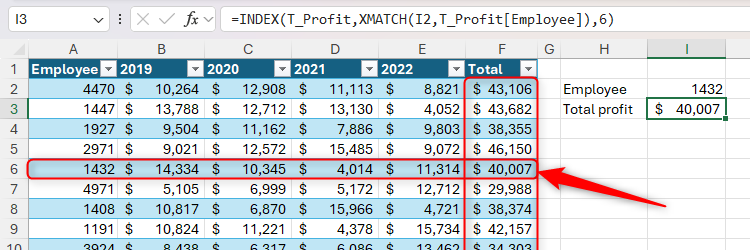
In this scenario, you don't need to enter the match type or search mode arguments for the XMATCH part of the formula, as the default settings return an exact match and look from top to bottom.

But what if you want to return the value from another column, such as an employee's profit in a given year? That's where two-way lookups come in handy.

Using INDEX With XMATCH for Two-Way Lookups

The benefit of using INDEX with XMATCH for two-way lookups is that you can change the parameters for your search without editing the formula. This is because XMATCH identifies both the row number and the column number, meaning you don't have to hardcode them into the formula.

Suppose you want to quickly find out how much profit employee 1191 made in 2021.



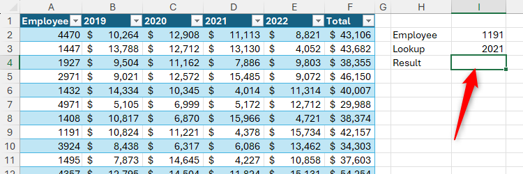
To do this, in cell I4, type:

=INDEX(T_Profit,XMATCH(I2,T_Profit[Employee]),XMATCH(I3,T_Profit[#Headers]))

where

• T_Profit is the name of the table where the value will be found,
• XMATCH(I2,T_Profit[Employee]) tells the INDEX function which row of the Employee column to look in, based on the value in cell I2, and
• XMATCH(I3,T_Profit[#Headers]) tells the INDEX function which column of the T_Profit table to look in, based on the value in cell I3.

If your column headers contain numerical values, like dates, you may see an #N/A error when you press Enter.



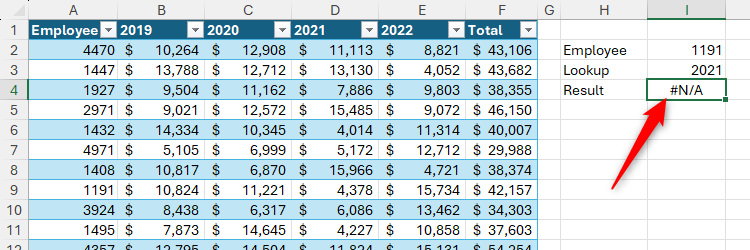
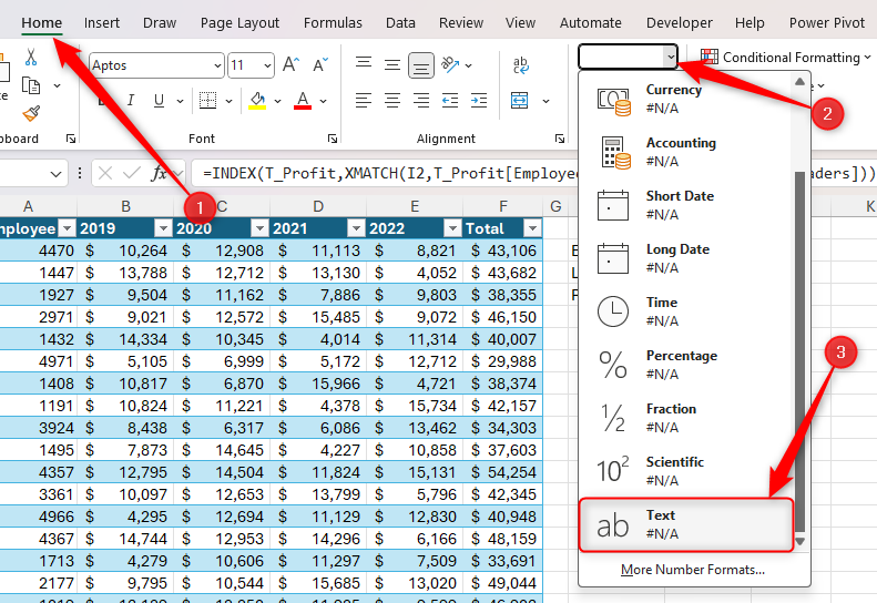
This is because Excel actually stores column headers as text, even if they appear numeric. So, to ensure you get a like-for-like match between the lookup value and the lookup array, select the cell containing the corresponding lookup value (which, in this example, is cell I3), and in the Home tab on the ribbon, click "Text" in the number format drop-down menu.



Then, select the cell containing the column lookup value (I3), press F2 to activate cell edit mode, and press Enter. Now, Excel sees both the lookup value and the lookup array as having the same number format, so the formula correctly returns the expected value.



Now, type different lookup parameters into cells I2 and I3, and see the formula return the corresponding result.



---

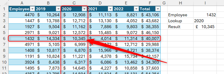
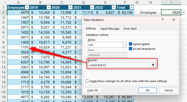
Now that you know how to use INDEX and XMATCH to perform two-way lookups, you could go one step further and use data validation to create drop-down menus in the cells containing the lookup values, further speeding up the lookup process and ensuring you don't accidentally enter an invalid value.

However, bear in mind that you can't use column headers as the source of a data validation list. To overcome this hurdle, enter direct cell references into the Source field of the Data Validation dialog box, or name the ranges and reference those instead.


Source

Source
Source: https://www.howtogeek.com/microsoft-excel-index-xmatch-perform-two-way-lookup/

This Excel Function Is So Much Smarter Than VLOOKUP

VLOOKUP has frustrated me with its rigid limitations and clunky syntax. But, not anymore. I found an Excel fucntion that handles lookups in any direction and offers precise matching control.

XMATCH Works in Any Direction You Want

The biggest frustration with VLOOKUP is its stubborn left-to-right requirement. If your lookup column isn't the leftmost in your range, you're stuck. You have to either rearrange your data or find a workaround. It can waste time restructuring spreadsheets just to make VLOOKUP happy.

Excel's XMATCH function eliminates this headache. Unlike VLOOKUP's rigid structure, XMATCH searches any array in any direction. You can find data to the left of your lookup column. You can also search vertically down a column or horizontally across a row; XMATCH handles both effortlessly.

Here's the basic syntax:

=XMATCH(lookup_value, lookup_array, [match_mode], [search_mode])

Let's break down these parameters:

• lookup_value: What you're searching for.
• lookup_array: The range where you're searching.
• match_mode: How exact your match needs to be (0 for exact, -1 for exact or next smallest, 1 for exact or next largest).
• search_mode: Which direction to search (1 for first to last, -1 for last to first, 2 for binary search).

Here's a practical example from an employee database. Say you need to find which department "Kristen Tate" works in, but the employee names are in column D while departments are in column B. With VLOOKUP in an Excel spreadsheet, this setup would force you to rearrange your data since you can't look left.

But you can use the XMATCH function to return her position in the name column as shown in the following formula:

=XMATCH("Kristen Tate", D:D, 0)

It changed my workflow as I no longer need to count columns. With VLOOKUP in an Excel spreadsheet, you're constantly counting to determine the column index number. If you add a new column to your data, suddenly your formulas break because the index numbers shift.

XMATCH Gives You Better Control Over Matching

VLOOKUP's matching options are limited to an exact match or an approximate match—that's it. If your data isn't perfectly clean, you're stuck spending time tidying up a messy Excel sheet before you can even start your lookup.

XMATCH makes it easy with its match_mode parameter. Set it to 0 for exact matches, just like VLOOKUP's FALSE parameter. But here's where it gets interesting. You can use -1 to find the exact match or the next smallest value, and 1 for the exact match or next largest value.

Consider salaries in the employee dataset. To find the employee earning closest to but not exceeding $75,000, you'd use:

=XMATCH(75000, H:H, -1)

This formula returns the position of the highest salary from column H that doesn't exceed your target value—something VLOOKUP struggles with unless your data is perfectly sorted.

The search_mode parameter adds another layer of control. While 1 searches from first to last (the default), -1 searches from last to first. This parameter matters when you have duplicate values and need the most recent entry.

For instance, if "John Smith" appears multiple times in column D of a dataset, we can use the following formula to find his last occurrence.

=XMATCH("John Smith", D:D, 0, -1)

Understanding these parameters helps you approach data lookup more effectively. This level of control means fewer helper columns and less data manipulation. Your formulas become more robust and your spreadsheets stay cleaner.

XMATCH Pairs Perfectly With INDEX

XMATCH proves more handy when you combine it with the INDEX function. While XMATCH finds the position, INDEX retrieves the actual value from that position. It's one of the useful Excel functions to find data quickly, but together, they create a more flexible lookup combination.

Here's the basic syntax when you combine both:

=INDEX(return_array, XMATCH(lookup_value, lookup_array, [match_mode]))

This pairing eliminates VLOOKUP's column-counting nightmare. Instead of remembering that salary is the eighth column, you simply specify the salary column directly. Hence, you don't get the broken formulas when you add or remove columns.

Let's say you need to find Kristen Tate's department from the employee data with INDEX and XMATCH:

=INDEX(R:R, XMATCH("Kristen Tate", D:D, 0))

The above formula reads naturally and returns a value from column R at the position where "Kristen Tate" appears in column D.

This combination also handles complex lookups, such as when you need the salary of the employee in the Sales department with the highest employee ID:

=INDEX(A:A, XMATCH(MAX(IF(R:R="Sales", H:H)), IF(R:R="Sales", H:H), 0))

This array formula finds the maximum employee ID within Sales, then returns that person's salary. If you were to try that with VLOOKUP, you'd need multiple helper columns and other workarounds.

XMATCH has completely replaced VLOOKUP in my workflow. The directional flexibility, precise matching control, and easy INDEX integration make it the lookup function that I needed the most. Once you experience this level of control, going back to VLOOKUP doesn't sound practical.

Source: https://www.makeuseof.com/xmatch-excel-function-vs-vlookup/