How to create simple and dependent drop-down lists

Using tables, named ranges, formulas, data validation, and table styles

Drop-down lists in Microsoft Excel (and Word and Access) allow you to create a list of valid choices that you or others can select for a given field. This is especially useful for fields that require specific information; fields that have long or complex data that’s hard to spell; or fields where you want to control the responses.
Creating dependent drop-down lists (when combined with an INDIRECT function) is another benefit. This allows you to select a product category from the main menu drop-down list box (such as Beverages), then display all the related products from the submenu (dependent) drop-down list box (such as Apple Juice, Coffee, etc.). This works very well for ordering and inventory purposes because it divides all the products into manageable categories. This is how most wholesale and retail companies handle their product lines. In fact, companies from hospitals and insurance carriers to banks and more use drop-down lists, check boxes, combo lists, and/or radio buttons to minimize typing and user errors.

How to create a simple drop-down list

We’ve created a sample drop-down list so you can practice the steps, or feel free to use your own data.

If your spreadsheet database is large or contains numerous fields, we recommend that you place the list box items in a table on a separate spreadsheet, but in the same workbook. However, if your list is relatively short, you can type the items for your list, separated by commas, in the Source field of the Data Validation dialog window.
1. Open a new workbook and add a second spreadsheet tab (click the ‘+’ sign at the bottom of the screen on the tab bar).
2. Rename Spreadsheet 1 as “wks” for worksheet, and Spreadsheet 2 as “lists.”
3. Enter the names of 10 doctors (or other applicable items) in column A from A1 through A10.
4. Sort the list to your preference. If you plan to sort by last name, enter the last name first, then the first name and middle initial on your original list.

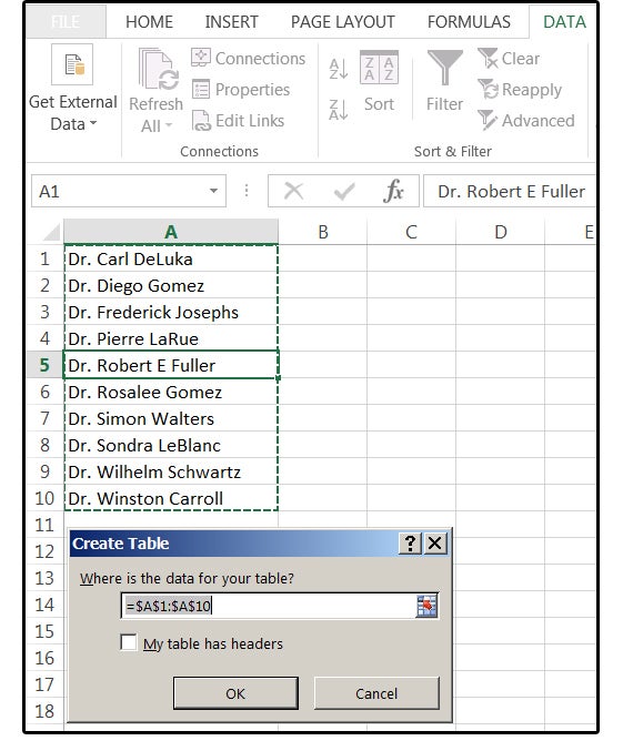
5. Highlight the range (A1:A10) or just position your cursor on any cell in the list, and press Ctrl+ T to convert this group of items to a table. Excel calls it Table 1, 2, 3, etc., which is not a problem if there is only one table. Be sure to check the box that says “My Table Has Headers.”
Note: When data is in a table, you can add or delete items from the list (and all other drop-down lists that use that same table) and they will all update automatically.

JD Sartain / IDG Worldwide

Enter your list of items, then convert the list to a table.

6. Move to Spreadsheet 1 (renamed wks). Enter some data similar to that shown in the following graphic, for example: Type of Surgery, Date, Time, and Surgeon, or create your own data.
7. Select the cell or group of cells where you want the drop-down list to appear. In this case, select D2 (or D2:D11, if you prefer, though it's not necessary to highlight the entire column).
8. From the Data tab, select Data Validation > Data Validation.
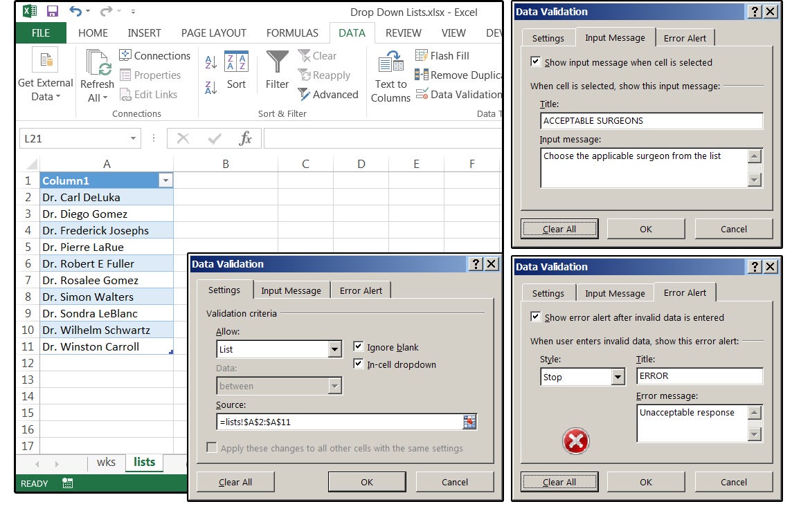
9. In the Data Validation dialog window, choose the Settings tab. In the Validation Criteria panel in the Allow field, select the option called List from the drop-down list box.

JD Sartain / IDG Worldwide

From the Settings tab, choose List from the list box.

10. Tab down to the Source field and click inside this box.
11. Move your cursor outside of this dialog window and select the lists spreadsheet from the workbook tabs at the bottom of the screen.

12. Highlight the range of doctors—that is, A2 through A11. Notice that Excel adds this range in the Source field box (=lists!$A$2:$A$11) for you.
13. Next, click the Input Message tab and enter a Title and Input Message for your drop-down list.
14. Next, click the Error Alert tab and enter the Title and Error Message for your drop-down list.
15. Click OK and your drop-down list box is complete.

JD Sartain / IDG Worldwide

Enter the Source range, Input Message, and Error Alerts for your drop-down list box.

16. Move back to the wks spreadsheet and position your cursor in cell D2. Notice the arrow for the drop-down list box, and your custom Input Message appears to the right of each cell in this column that you select. Click the down arrow and choose a doctor from the list that specializes in the type of surgery on the corresponding row of column A. For example, Dr. Simon Walters’ field is hip surgery.
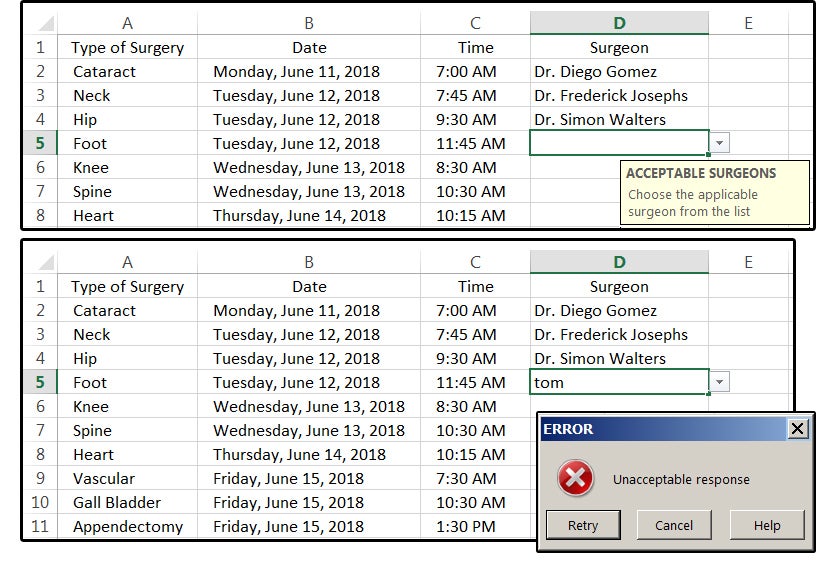
17. If anyone types an invalid name—that is, they try to type in a name that is not on the Acceptable Surgeon’s list, the custom error message that you specified appears when the Enter key is pressed. Click Cancel to exit this dialog.

JD Sartain / IDG Worldwide

Choose a doctor from the list or type an invalid entry for an Error Alert.

Create dependent drop-down lists
Dependent drop-down lists are like the submenus in Office applications. The main menu (or drop-down list) displays various options with submenus below each one that display further options related to the main menu. In our sample worksheet, the drop-down list provides a selection of surgeons for you to choose that matches the type of surgery scheduled.
For this next exercise, imagine that you run a small rural hospital located about 50 miles from a large city that has three large, completely staffed hospitals. It’s your job to schedule surgeons from one of these three large facilities to see patients at your hospital. The “main” drop-down list contains a selection of hospitals (by location) where each surgeon practices. The submenu drop-down lists provide the names of each surgeon that works in each of these facilities: East Side, West Side, or Midtown.

A. Create the lists

1. First, add another spreadsheet and name it lists2.
2. On the lists2 spreadsheet, enter the following title for column A: Hospital Locations. Under Hospital Locations enter the names EastSide, WestSide, and Midtown in cells A2, A3, and A4, respectively (without spaces or use one word).
3. Move your cursor to the first cell under the title Hospital Locations (A2). Click Home > Format As Table, and choose a Table Style from the submenu, then click OK.
4. Select the hospital locations in this list (A2:A4). Enter a table name (Locations) in the Name box (above column A) or press Ctrl+ T to convert these items to a table, which Excel names Table 1, 2, 3, etc. Finally, check the box that says My Table Has Headers.
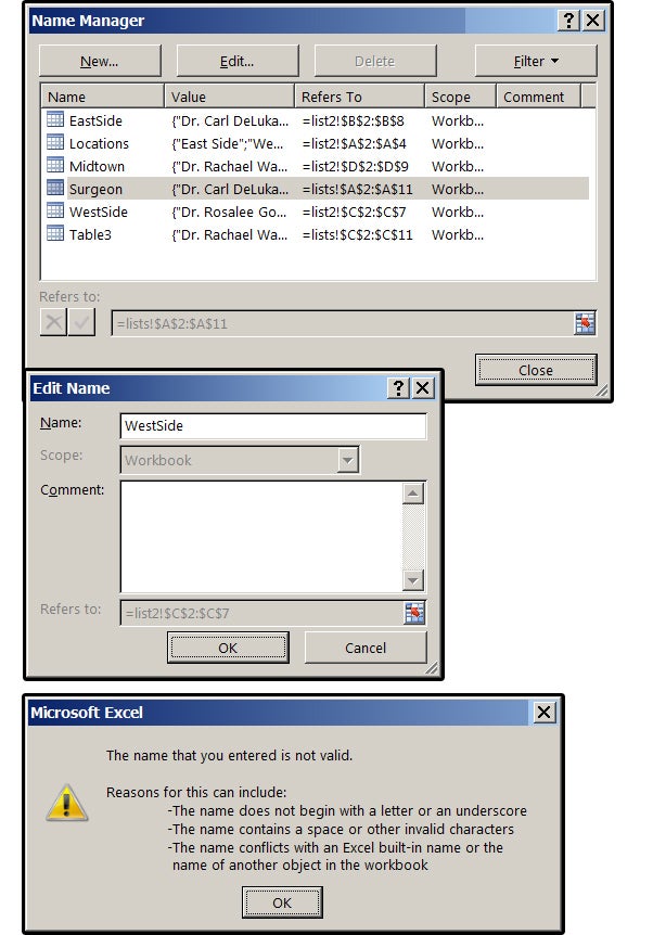
5. To rename your tables, select Formulas > Name Manager. Cursor down to Table 1 (2, 3, 4, etc.), then click the Edit button.
6. In the Edit Name dialog box, type in the new name (Locations).
Note: Excel does not allow spaces or other special characters. Names must begin with a letter or an underscore, and names cannot conflict with any of Excel’s built-in names or other objects in the workbook (for instance, you cannot have two ranges with the same name in a single workbook—even if the ranges are in separate spreadsheets).

JD Sartain / IDG Worldwide

Rename your tables using Excel’s Name manager.

7. Next, you must create a separate table for each of the hospital locations. On the lists2 spreadsheet, enter the following titles, for column B: East Side, C: West Side, and D: Midtown (these column labels will also be your range names minus the spaces).
8. Enter some doctors' names under each of these three columns (B, C, D).
9. Format each list as a named table (repeat step 3 above).
10. Highlight the range of each column individually (B1:B8; C1:C7; D1:D9). Press Ctrl+ T to convert these groups of items to Tables, which Excel names Table 2, 3, 4, etc., then check the box that says My Table Has Headers. Repeat steps 5 and 6 above to rename your tables. Remember, no spaces in range names.

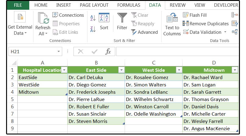JD Sartain / IDG Worldwide

Create tables for your lists.

Note: If you have multiple tables, name them based on the header you provided for each column.

B. Create the drop-downs

1. First, return to the wks spreadsheet and delete the previous drop-down list in column D titled Surgeons. Create a new header in column D1 titled Location, and name column E1 Surgeons.
2. Select cells D1:E11, then select Home > Format As Table, choose a style, check the headers box, and click OK.
3. Next, select cells (D2:D11) for the main menu drop-down list.
4. From the Data tab, select Data Validation > Data Validation.
5. In the Data Validation dialog window, choose the Settings tab. In the Validation Criteria panel in the Allow field, select the option called List from the drop-down list box.
6. In the Source box, click the list2 spreadsheet, highlight the Hospital Location list minus the header (A2:A4), and click OK.

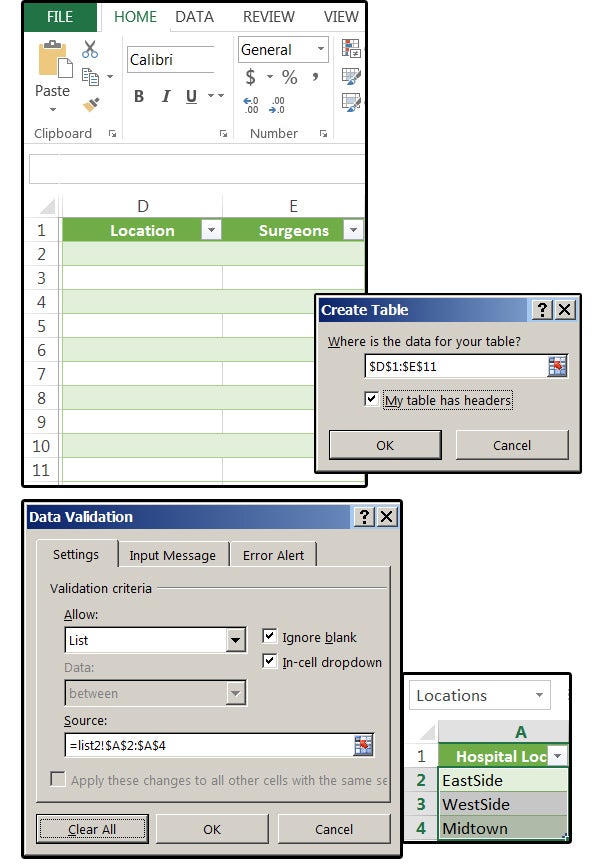JD Sartain / IDG Worldwide

Create the main menu drop-down list.

7. Move your cursor to cell E2.
8. Repeat steps 8 and 9 above.
9. This time, in the Source box, enter this formula: =INDIRECT($D$2)—but this is for the current cell only—then click OK.
Note: If you receive the Source Error message, just click Yes, because the errors will cease when the data from the drop-down lists fill in.
10. To fill out the column (which is the obvious course), enter the formula like this: =INDIRECT($D2)—yes, without the '$' sign on the row number—then copy cell D2 down from D3 through D11. This activates the entire range.

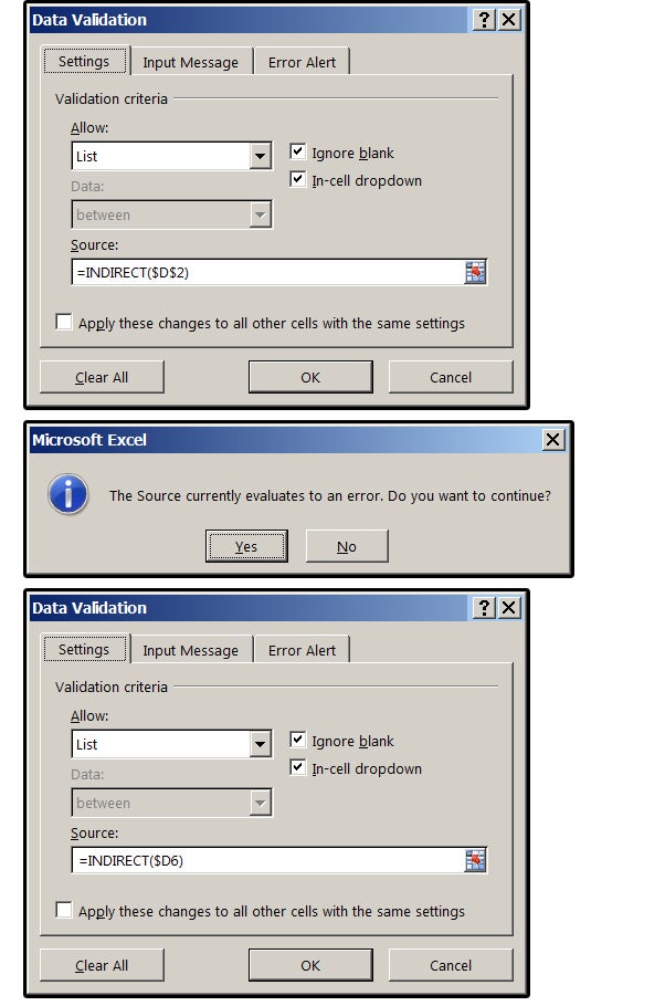JD Sartain / IDG Worldwide

Enter the INDIRECT function as a relative formula, then copy.

11. If you want to add an Input Message or an Error Alert, repeat steps 13 through 14 above in the section "How to create a simple drop-down List."

C. Test your work

Now it’s time to test your work. Click the drop-down arrows (one at a time) in column D (Location).
1. Choose a hospital from the list, and it appears in the active cell.
2. Move your cursor to column E (Surgeon) and choose a doctor from the list of doctors at the location you specified in column D.

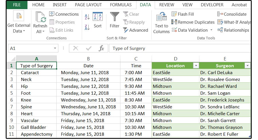JD Sartain / IDG Worldwide

The drop-down lists work as expected.

D. Work-around for two word items

If you want to use two or more words for the main menu drop-down (e.g., Location) and you do not want to run the words together without a space (e.g., East Side instead of EastSide), enter this formula in the dependent drop-down (Surgeon) Source box in the Data Validation dialog window:

=INDIRECT(SUBSTITUTE(D2," ","")) where D2 is the cell address, " " means quote-space-quote, and "" means quote-quote with no space. Translation: substitute cell D2 that has a space with D2 minus the space.
That’s all for now. If you need additional help, you can download this spreadsheet here:

Source: https://www.pcworld.com/article/3276341/office-software/excel-how-to-create-simple-and-dependent-drop-down-lists.html